Lesson Part 1

Introduction

We begin by studying Rolle's theorem, which led mathematicians to the mean value theorem.

Michel Rolle was a French mathematician (1652-1719).

The following four diagrams illustrate his theorem:

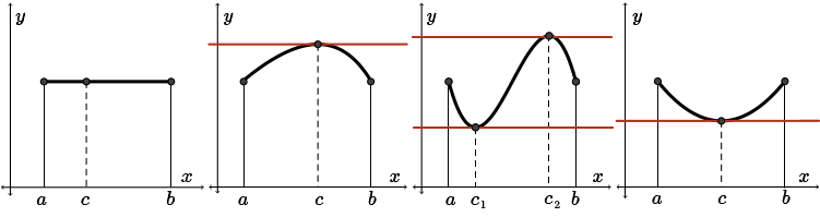
Image Description:

1. The first function is a horizontal line between the interval. All points have a horizontal tangent.
2. The second function curves upwards between the interval. There is a horizontal tangent at the maximum.
3. The third function has a sideways “S-bend” shape between the interval. There is a horizontal tangent at the minimum and a horizontal tangent at the maximum.
4. The fourth function curves downwards between the interval. There is a horizontal tangent at the minimum.

In each diagram, we have a continuous function, \(f\), that is bounded by the closed interval \([a,b]\) with the \(y\)-value at \(a\) equal to the \(y\)-value at \(b\). Notice that the height above the \(x\)-axis of each endpoint on the graph is equal; i.e., \(f(a)=f(b)\).

Each function is differentiable within the open interval \((a,b)\).

In the four diagrams, we see that within each open interval, there is at least one point \(x=c\) where \(f'(c )=0\). In other words, there exists at least one point where the tangent is horizontal. It was this idea that led to Rolle's theorem.

Mean Value Theorem

Rolle's Theorem

If \(f\) is a continuous function on the closed interval \([a,b]\), and \(f\) is differentiable on the open interval \((a,b)\), and \(f(a)=f(b)\), then there exists a value \(x=c\) in \((a,b)\), such that \(f'(c )=0\).

In other words, there must be at least one point where the slope of the tangent is horizontal.

Following from Rolle's theorem, another French mathematician, Joseph-Louis Lagrange, connected the average rate of change of a function over an interval with the instantaneous rate of change of the function at a point within the interval. His ideas lead to the mean value theorem.

Mean Value Theorem

If \(f\) is a continuous function on the closed interval \([a,b]\), and \(f\) is differentiable on the open interval \((a,b)\), then there exists a value \(x=c\) in the open interval \((a,b)\), such that the instantaneous rate of change at \(x=c\) is equal to the average rate of change from \(a\) to \(b\). That is,

\[ f'( c) = \dfrac{f(b)-f(a)}{b-a}\]

Essentially what Lagrange is trying to say is that, if we were to calculate the slope of the secant between each endpoint of the closed interval, there would exist another point within the closed interval whose tangent has the same slope as the secant.

The following diagrams illustrate two cases of the mean value theorem:

In both diagrams, we see that the secant \(AB\) is parallel to the tangent line at one or more points within the closed interval. Since these two lines are parallel, they must have the same slope.

Lesson Part 2

Examples

Let's now use an example to confirm that the mean value theorem holds true for a function.

Example 1

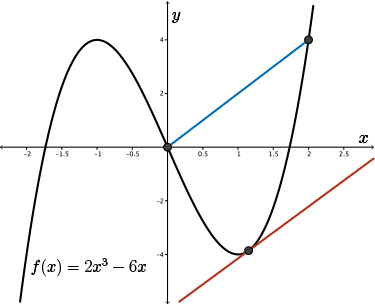
Confirm that the mean value theorem holds true for the function \(f(x)=2x^3-6x\) on the closed interval \([0,2]\).

Solution

Let's begin by calculating the average rate of change (ROC) of the function \(f(x)=2x^3-6x\) on the closed interval \([0,2]\). Recall that the average rate of change is found by \(\frac{\Delta{y}}{\Delta{x}}\).

\begin{align*} \text{Average ROC} & = \dfrac{f(2)-f(0)}{2-0} \\ & = \dfrac{2(2^3)-6(2) -\left [ 2(0)^3 -6(0) \right ]}{2-0} \\ & =\dfrac{4}{2} \\ & =2 \end{align*}

So to confirm that the mean value theorem holds true for this function, we will now confirm that there exists a point \(c\) in \((0,2)\), where the tangent at \(c\) has slope \(2\).

In other words, we are looking for an instantaneous rate of change within the open interval \((0,2)\) that is equal to the average rate of change, which is \(2\).

(Note that \(f(x)\) is continuous on \([0,2]\) and \(f(x)\) is differentiable on \((0,2)\) and so the hypotheses of the mean value theorem hold.)

The derivative of \(f(x)\) is \(6x^2-6\).

Now we substitute \(f'(c ) = 2\) into this function for the derivative to see if a tangent exists with this slope.

The theorem requires that there is an \(x=c\) such that

\(f'(c ) =\dfrac{f(2)-f(0)}{2-0} =2\)

Thus, we let \(f' (c ) =2\) and solve for \(c\).

\begin{align*} 6c^2-6 &=2\\ c^2 &= \dfrac{8}{6} \\ c &= \pm \sqrt{\dfrac{4}{3}} \\ c&= \pm \dfrac{2\sqrt{3}}{3} & \text{reduced and rationalized}\\ c & \approx \pm 1.15 \end{align*}

Since \(1.15\) is within the open interval \(0 \lt x \lt 2\), a tangent to the curve \(y=f(x) = 2x^3-6x\) with slope \(2\) exists within this open interval at \(x=c = \frac{2\sqrt{3}}{3}\). Thus, this example confirms the mean value theorem.

We can check our result by examining the following graph. Notice how the slope of the tangent, the red line, is equal to the slope of the secant, the blue line.

The mean value theorem provides us with information about a function from its derivative.

We can use this information to make predictions about the function's graph, which we will see in the next module.

Let's now use the mean value theorem to make some conclusions about a function.

Example 2

Suppose a function, \(f\), is differentiable for all \(x\in\mathbb{R}\) and has \(f(0) = -5\). If \(f'(x) \leq 7\) for all values of \(x\), use the mean value theorem to determine the largest possible value of \(f(2)\).

Solution

The mean value theorem guarantees that there exists \(x=c\) in \((0,2)\) such that \(f'(c )\) is equal to the average rate of change between the end points of this interval. In other words,

\[f'(c ) = \dfrac{f(2)-f(0)}{2-0}\]

Thus,

\begin{align*} 2f'(c )&= f(2)-f(0) \\ f(2) &=2f'(c ) +f(0) \end{align*}

Since \(f(0)=-5\) and \(f'(x) \leq 7\) for all real \(x\), we have

\begin{align*} f(2) &=2f'(c ) +f(0) \\ &\leq 2(7)+(-5) \\ &= 9\end{align*}

Therefore, the largest possible value that \(f(2)\) could be is \(9\).

Quiz

See the quiz in the side navigation.