Lesson Part 1

Introduction

Given a function \(f(x)\), a quick way to get an idea of its behaviour is to sketch the graph of \(y=f(x)\).

This is often done by plotting discrete points and then connecting the points with a smooth curve.

The uncertainty in this approach is clear if one asks the following reverse question.

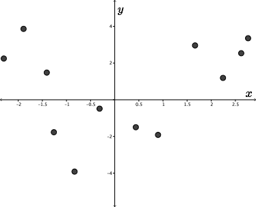
Given a discrete set of points \((x,y)\), what might be the behaviour of a corresponding function \(f(x)\)?

Consider the graph shown on the screen. How would we connect these points?

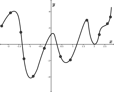
Would the function look like this?

Or would the function look like this?

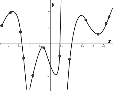
There are many possibilities!

Even if we know the function \(f(x)\) and use a sophisticated computer graphing tool, there is no guarantee that the resulting graph will reveal all the essential features of the function.

Consider these computer generated plots of the function

\[y= \dfrac{x-3}{\sqrt{5x+1}-\sqrt{3x+7}}\]

The function is actually undefined at \(x=3\), where it has the indeterminate form \(\frac{0}{0}\).

Yet even if we ask the graphing program to zoom in on a small interval about that point, it does not reveal this fact.

One must always keep in mind that computers plot a discrete set of points and make assumptions about the function's behaviour between these points.

Thus, caution is advisable with curve sketching.

We need the methods of calculus to analyze \(f(x)\) first and to generate a sketch of \(y=f(x)\) which accurately portrays the essential qualitative features of \(f\).

This process will be the focus of this unit.

Then, if needed, we can confidently use computers to generate quantitative information, knowing the relevant intervals of \(x\) and \(y\) and the points where special care is needed.

In this module, students will explore how the first derivative can give us evidence as to the behavior of a graph.

Lesson Part 2

Intervals of Increase and Decrease of a Function

A function, \(f\), is increasing over an interval if the graph, \(y=f(x)\), rises from left to right; in other words, if \(y\) increases as \(x\) increases.

The definition of an increasing function is as such.

A function is increasing on an interval \(I\) if, for any pair of points, \(x_1 \lt x_2\) in \(I\), \(f(x_1) \lt f(x_2)\).

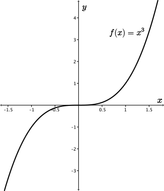
For example, let's consider the graph of \(y=f(x)=x^3\). When we consider this graph from left to right, we see that the value of the points increase throughout its domain.

Consider a tangent line drawn to any point along the graph of \(y=f(x)=x^3\).

Except for at \(x=0\), every tangent line drawn to this curve will have a positive slope.

This means that \(f'(x) \gt 0\) for all \(x\in\mathbb{R}\) where \(x\neq 0\).

When \(x=0\), \(f'(0)=0\), so there is a critical point at \(x=0\) with a horizontal tangent line to \(y=x^3\) at \((0,0)\).

Clearly, the graph \(y=f(x)\) will be increasing whenever the tangent line to the graph has a positive slope, provided a tangent line exists. Thus, we have property 1.

Property 1: If \(f'(x) \gt 0\) for all \(x\) in an interval \(I\), then \(f(x)\) is increasing on \(I\).

For example, consider the function \(f(x)=x^3\).

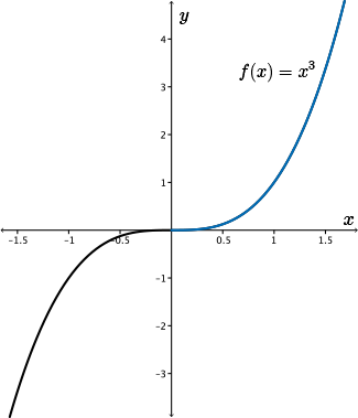
The derivative is \(f'(x)=3x^2\), and so \(f'(x)\) is positive for all \(x \neq 0 \).

In particular, we have \(f'(x) \gt 0\) for all \(x \gt 0\) and so by property 1, \(f(x)\) must be increasing on the entire interval \(x\gt 0\).

This property is confirmed by looking at the graph of \(f(x)\) on \(x \gt 0\).

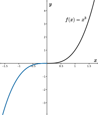
Similarly, we have \(f'(x)\gt 0\) for all \(x\lt 0\) and so \(f(x)\) must be increasing on the entire interval \(x\lt 0\) as well.

This is also confirmed by looking at the graph of \(f(x)\) on \(x\lt 0\).

What can be said about an interval containing the point \(x=0\)?

We cannot have \(f'(x)\gt 0\) for an interval containing \(x=0\), but \(f(x)\) is in fact increasing over these intervals as well.

This example shows that the converse of property 1 is not true.

Converse of Property 1: If \(f(x)\) is increasing on an interval \(I\), then \(f'(x) \gt 0\) for all \(x\) in \(I\).

From the graph, we can see that \(f(x)=x^3\) is increasing on its entire domain. In particular, it is increasing over the interval \((-1,1)\). We can see this by simply comparing function values on this interval.

However, since this interval contains \(x=0\) and \(f'(0)=0\), we do not have \(f'(x)\gt 0\) for all \(x\) in \((-1,1)\).

Therefore, the converse of property 1 does not hold in general. In other words, functions can still be increasing over an interval even if the tangent lines don't all have positive slopes.

It is also possible that \(f'(x)\) does not exist but \(f\) is still increasing or decreasing. Let's consider this case in the next example.

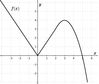
For example, consider the function

\(\begin{align*} f(x) = \begin{cases} \dfrac{3}{2} \lvert x \rvert &\text{ for } x\leq 2 \\ & \\ (5-x)(x-1) &\text{ for } x \gt 2\end{cases}\end{align*}\)

which increases on \(0 \lt x \lt 3\), yet \(f'(2)\) does not exist since the slope is \(\frac{3}{2}\) to the left of \(x=2\), but approaches \(3\) from the right.

Lesson Part 3

Intervals of Increase and Decrease of a Function

A function, \(f\), is decreasing over an interval if the graph, \(y=f(x)\), falls from left to right; in other words, if \(y\) decreases as \(x\) increases.

The definition of a decreasing function is as follows.

A function is decreasing on an interval \(I\) if, for any pair of points, \(x_1 \lt x_2\) in \(I\), \(f(x_1) \gt f(x_2)\).

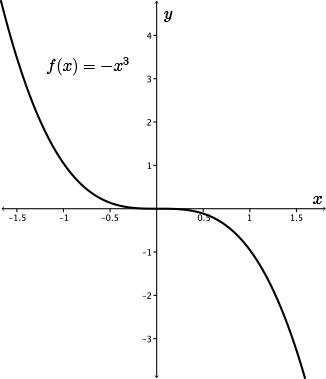
For example, let's consider the graph of \(y=f(x)=-x^3\). This function decreases through its domain.

Consider a tangent line drawn to any point along the graph of \(y=f(x)=-x^3\).

Except for \(x=0\), every tangent line drawn to this curve will have a negative slope.

This means that \(f'(x) \lt 0\) for all \(x \in \mathbb{R}\) where \(x\neq 0\).

At \(x=0\), \(f'(0)=0\), and the tangent line to \(y=-x^3\) is horizontal at \((0,0)\).

Clearly, the graph of \(y=f(x)\) will be decreasing whenever the tangent line to the graph has a negative slope, if a tangent exists. Thus, we have property 2.

Property 2: If \(f'(x) \lt 0\) for all \(x\) in an interval \(I\), then \(f(x)\) is decreasing on \(I\).

For example, consider the function \(f(x)=-x^3\).

The derivative is \(f'(x)=-3x^2\).

In particular, we have \(f'(x)\lt 0\) for all \(x\neq 0\) and so \(f(x)\), by property 2, must be decreasing on the intervals \(x\gt 0\) and \(x\lt 0\).

This is confirmed by looking at the graph of \(f(x)\) on each of these intervals.

What can be said about an interval containing \(x=0\)?

Again, we show that the converse of property 2 does not hold in general. Here's the statement of the converse.

Converse of Property 2: If \(f(x)\) is decreasing on an interval \(I\), then \(f'(x)\lt 0\) for all \(x\) in \(I\).

Is this always true?

We can see that \(f(x)=-x^3\) is decreasing on its entire domain. Again, we can see this by simply comparing function values. In particular, it is decreasing over the interval \((-1,1)\).

But since this interval contains \(x=0\) and \(f'(0)=0\), we do not have \(f'(x) \lt 0\) for all \(x\) in \((-1,1)\).

Therefore, the converse to property 2 does not hold in general. This means that functions can still be decreasing over an interval even if the tangent lines don't all have negative slopes.

Investigation

See the investigation in the side navigation.

Lesson Part 4

Investigation Discussion

From the investigation, we see that critical points (points where \(f'(x) =0\); in other words, the slope of the tangent is horizontal, or points where \(f'(x)\) does not exist) separate the intervals of increase from the intervals of decrease.

Let's now use our knowledge of the intervals of increase and decrease and critical points to complete the following example.

Examples

Example 1

With the aid of graphing technology, find where the function \(f(x)=x^5-5x^3+5x^2\) is increasing and where it is decreasing.

Solution

To begin, let's graph this function.

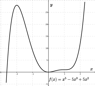
Beginning at the left side of the graph, we see that, initially, the \(y\)-values rise as we move towards the right.

Therefore, the graph is increasing.

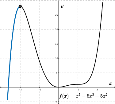
At \(x=-2\), we reach a critical point having a horizontal tangent.

As we continue to move towards the right, the \(y\)-values now fall and thus the graph is decreasing.

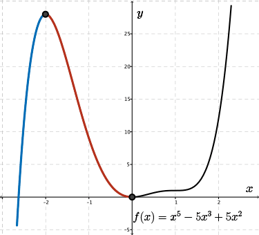
The next critical point reached is at \(x=0\).

After this critical point, the \(y\)-values begin to rise again, so \(f(x)\) is increasing.

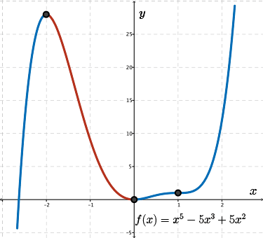
The final critical point is at \(x=1\); however, unlike the behaviour of critical points previously seen, the graph remains increasing for \(x\gt 1\).

In summary, \(f(x)\) increases on the intervals \(x \lt -2\) and \(x\gt 0\), while \(f(x)\) decreases in the interval \(-2 \lt x\lt 0\).

Now, you may be asking yourself, “but how do we determine intervals of increase and decrease algebraically?” We will use the first derivative test to find these.

Lesson Part 5

The First Derivative Test: Determining Intervals of Increase and Decrease Algebraically

We have seen that critical points separate the intervals of increase from the intervals of decrease.

Also, if the value of the derivative is positive, i.e., \(f'(x)\gt 0\), then \(f(x)\) is increasing, and if the value of the derivative is negative, i.e., \(f'(x) \lt 0\), \(f(x)\) is decreasing.

To algebraically determine a function's intervals of increase and decrease, we first need to determine the positions of the critical points. This will tell us the possible boundaries of each interval of increase or decrease.

Then, we will test points inside these intervals to determine if the slope of the tangent is positive or negative, which tells us if \(f(x)\) is increasing or decreasing.

Let's try this method for the function we previously saw in the example: \(f(x)=x^5-5x^3+5x^2\).

This function is a polynomial and therefore it is differentiable for all points within its domain, \(x\in\mathbb{R}\).

Thus, the critical points will only occur when \(f'(x)=0\), since there are no points on the curve where \(f'(x)\) does not exist.

The first derivative gives another polynomial function:

\[f'(x) = 5x^4-15x^2+10x\]

Since the critical points to this curve will occur when \(f'(x)=0\), we solve this equation for \(x\), and we get

\(\begin{align*} 0&= 5x^4-15x^2+10x \\ 0&=5x(x^3-3x+2) \end{align*}\)

Using the factor theorem (to solve for \(x\)), when \(x=1\), we see that the quantity inside the brackets equates to the following: \(x^3-3x+2 = (1)^3 -3(1) +2 =0\).

Therefore, the expression \(x^3-3x+2\) has a factor \((x-1)\).

Now that we have identified a factor of this expression, using synthetic or long division, divide \(x^3-3x+2\) by \((x-1)\) to get \(x^2+x-2\).

Thus, when we set \(f'(x)=0\), we see that \(f'(x)\) can be factored as follows:

\(\begin{align*} 0 &=5x(x-1)(x^2+x-2) \\ 0& = 5x(x+2)(x-1)^2 \end{align*}\)

Therefore, critical points occur at \(x=-2\), \(0\), and \(1\).

These will serve as the boundary points for our intervals.

Let's summarize the required information in a table. Start by arranging the critical points from least to greatest. Once you've arranged the critical points from least to greatest, now make the possible intervals of increase and decrease, starting with the smallest value.

So beginning at \(x = -2\), we have the interval \(x\lt-2\). The next largest critical point is \(0\), so the next possible interval will be \(-2 \lt x\lt 0\). In other words, \(-2\) is less than \(x\), which is less than \(0\).

Finally, the last critical point is at \(1\), so we have the following two intervals. We have when \(0 \lt x \lt 1\), in other words, \(0\) is less than \(x\), which is less than \(1\). And the last interval is for values where \(x\gt 1\).

This gives us a table with four column intervals: \(x\lt-2\), followed by \(-2 \lt x\lt 0\), followed by \(0 \lt x \lt 1\), and finally \(x\gt 1\). We then create two header rows: one for the derivative of the function, labelled \(f'(x)\), where we indicate whether this is positive or negative in the interval, and one for the function, labelled \(f(x)\), where we indicate whether this is increasing or decreasing as a result of our findings for \(f'(x)\).

Now, we test if \(f'(x)\) is positive or negative within these intervals.

Choose a value of \(x\) within the first interval, say \(x=-3\).

Now remember, as we are only interested if \(f'(x)\) is positive or negative. So you don't actually have to compute this value, we just need to show if this value would be positive or negative.

Substituting \(x=-3\) into \(f'(x)=5x(x+2)(x-1)^2\), we get \(f'(-3)=5(-3)[(-3)+2][(-3)-1]^2\).

Or more simply, we can just consider the sign of each factor: \(f'(-3) = (+)(-)(-)(+) = (+)\).

Therefore, \(f'(x) \gt 0\) and the function is increasing.

Putting this information for \(f(x)=x^5-5x^3+5x^2\) in the table, it confirms the behaviour we previously saw in the original graph when we completed the example.

	\(x\lt-2\)	\(-2 \lt x\lt 0\)	\(0 \lt x \lt 1\)	\(x\gt 1\)
\(f'(x)\)	\(f'(x)\gt 0\)	\(f'(x) \lt 0\)	\(f'(x) \gt 0\)	\(f'(x) \gt 0\)
\(f(x)\)	Increasing	Decreasing	Increasing	Increasing

You should see that when \(-2 \lt x\lt 0\), \(f'(x) \lt 0\), meaning that \(f(x)\) is decreasing within this interval. When \(0 \lt x \lt 1\), \(f'(x) \gt 0\). So we know that \(f(x)\) is increasing within this interval. And finally, when \(x\gt 1\), \(f'(x) \gt 0\), and so \(f(x)\) is increasing inside this interval.

We say that \(f(x)\) has a turning point at \(x=a\) if \(f(x)\) is continuous at \(x=a\) and \(f(x)\) changes from increasing to decreasing or from decreasing to increasing at that \(x=a\).

Note:
In the previous example, \(f(x)\) has turning points at \(x=-2\) and \(x=0\), but not at \(x=1\). The sign of \(f'(x)\) changes at \(x = -2\) and \(x = 0\), but does not change at \(x = 1\). That is, only two of the three critical points are also turning points of the function.

Lesson Part 6

The First Derivative Test: Determining Intervals of Increase and Decrease Algebraically

Critical points also occur for values of \(x\) in the domain of \(f\) where \(f'(x)\) does not exist.

In our discussion of differentiability, we saw that a function is not differentiable at \(x\) if any of the following 3 conditions hold.

1. \(f(x)\) has a discontinuity (infinite discontinuity i.e., vertical asymptote; removable discontinuity i.e., hole; jump discontinuity) or if \(f(x)\) has an end-point due to a restriction on its domain.

2. \(f(x)\) is continuous but there is no tangent line to the graph of \(y=f(x)\) at \(x=a\). This happens if the derivative \(f'(x)\) approaches a different value as \(x\) approaches \(a\) from the left and from the right.

   For example, consider the following three functions that are not differentiable at \(x=0\).

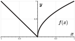
   First, we see a graph of \(f(x)=\lvert x \rvert\).

   

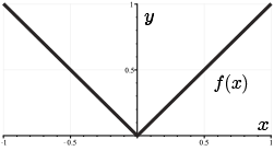
   At \(x = 0\), we have what we call a corner. Notice, that \(f'(x)\to -1\) as \(x\to 0^-\). However, \(f'(x)\to 1\) as \(x \to 0^+\). So here, the derivative values do not agree on either side, and so \(f(x)\) is not differentiable at \(x = 0\).

   In the second graph, we see an example of a cusp. This is the function \(f(x)=x^\frac{2}{3}\).

   

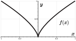
   Here, \(f'(x) \to -\infty\) as \(x\to 0^-\). And \(f'(x) \to +\infty\) as \(x\to 0^+\). So here, from either side, as we approach \(x = 0\), the tangent lines become very close to vertical and the function seems to curve back on itself.

   In the final example, we see a piecewise function that combines properties from our first two graphs. Here, the function is \(f(x)= \begin{cases} -x, &x\lt 0 \\ \sqrt{x}, &x\geq 0\end{cases} \).

   

   Here, we see that \(f'(x) \to -1\) as \(x\to 0^-\). In fact, it's constant at \(-1\) on the left-hand side. However, \(f'(x)\to \infty\) as \(x\to 0^+\). Here, again, our curve is not differentiable at the point \(x = 0\). In this case, we would also say that this graph has a corner at \(x = 0\).

3. \(f(x)\) is continuous and there is a tangent line to \(y=f(x)\) at \(x=a\), but the tangent line is vertical (infinite slope).

   Here, consider the following familiar example \(y = \sqrt[3]{x}\).

   

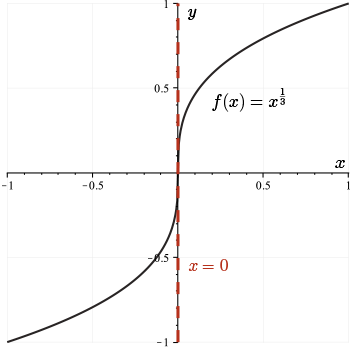
   At \(x = 0\), we have a tangent line, but the slope is infinite. And so this function does not have a derivative at \(x = 0\).

Lesson Part 7

The First Derivative Test: Determining Intervals of Increase and Decrease Algebraically

Let's examine why a vertical asymptote may divide intervals of increase from decrease of \(f(x)\).

In our discussion of continuity, we saw that at a vertical asymptote \(f(x)\) can approach the \(+\infty\) (or \(-\infty\)) from both the left side and right side of the vertical asymptote, or \(f(x)\) can approach \(+\infty\) from one side and \(-\infty\) from the other side.

The four possible cases are shown in the following diagrams.

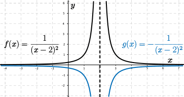
In the first diagram, we see that \(f(x)=\dfrac{1}{(x-2)^2}\) increases until \(x=2\), where it meets a vertical asymptote, and then \(f(x)\) decreases after this vertical asymptote. Also, \(g(x)=-\dfrac{1}{(x-2)^2}\) decreases until \(x=2\), and then after this vertical asymptote, it increases.

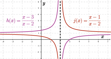
In the second diagram, \(h(x)=\dfrac{x-3}{x-2}\) increases for the entire domain, except when undefined at the vertical asymptote \(x=2\). And \(j(x)=\dfrac{x-1}{x-2}\) decreases for the entire domain, except when undefined at \(x=2\).

We see that a vertical asymptote can define the intervals where a function is increasing or decreasing, i.e., \(f'(x)\) may change sign at a vertical asymptote, or it may not.

Thus, when using the first derivative test, we proceed as follows:

1. Locate any discontinuities of \(f\) (vertical asymptote, removable or jump discontinuity) and any end-points of the domain of \(f\).
2. Find any critical points (i.e., points \((c,f(c ))\) where \(c\) is in the domain of \(f\), and \(f' (c )=0\) or \(f' ( c)\) is undefined).
3. Use these points to define intervals of \(x\)-values, and check the sign of \(f'(x)\) within each interval to determine whether \(f\) is increasing or decreasing.

It is helpful to use the table shown previously to summarize your information.

Lesson Part 8

Examples

Example 2

Find the intervals of increase and decrease for the function \(f(x) = \dfrac{x^2-2x}{(x-1)^2}\).

In this case, I would like you to use an algebraic approach.

Solution

First, we find any discontinuities of \(f(x)\).

Since \(x - 1\) appears in the denominator but not the numerator, we see that \(f(x)\) has a vertical asymptote at \(x=1\) but is continuous at every point in its domain \((x\neq 1)\).

Next, we locate any critical points of \(f(x)\).

Taking the derivative gives

\(\begin{align*} f'(x) &= \dfrac{(2x-2)[(x-1)^2]-(x^2-2x)[2(x-1)(1)]}{[(x-1)^2]^2} & \text{using quotient and chain rules} \\ &= \dfrac{2(x-1)^3-2x(x-2)(x-1)}{(x-1)^4} \\ &= \dfrac{2(x-1)[(x-1)^2-x(x-2)]}{(x-1)^4} & \text{common factors}\\ &= \dfrac{2(x^2-2x+1-x^2+2x)}{(x-1)^3} \\ &= \dfrac{2}{(x-1)^3} \end{align*}\)

Since critical points to this curve may occur when \(f'(x)=0\), solve for \(x\) in the equation

\[0 = \dfrac{2}{(x-1)^3}\]

There are no values of \(x\) that satisfy this equation.

Thus, the only point where \(f'(x)\) may change its sign is at the vertical asymptote \(x=1\).

Let's now complete the table for the first derivative test, noting that \((x-1)^3 \gt 0\) if \(x \gt 1\) and \((x-1)^3 \lt 0\) if \(x\lt 1\), so our intervals are when \(x\lt 1\) and when \(x \gt 1\).

Substituting a value where \(x\lt 1\) into the expression \(f'(x)\), we see that \(f'(x) \lt 0\), so \(f(x)\) is decreasing. When we substitute a value of \(x \gt 1\) into the expression for \(f'(x)\), we see that \(f'(x) \gt 0\), therefore \(f(x)\) is increasing within this interval.

So we get the following table for \(f(x) = \dfrac{x^2-2x}{(x-1)^2}\):

	\(x\lt 1\)	\(x \gt 1\)
\(f'(x)\)	\(f'(x) \lt 0\)	\(f'(x) \gt 0\)
\(f(x)\)	Decreasing	Increasing

In summary, \(f(x)\) is decreasing for \(x\lt 1\), and \(f(x)\) is increasing for \(x\gt 1\).

Lesson Part 9

Examples

If you feel ready for more of a challenge, let's now consider the following problem.

Challenge Problem

Suppose that \(f(x)\) and \(g(x)\) are positive differentiable functions such that \(f(x)\) has a local maximum and \(g(x)\) has a local minimum at \(x=c\). Prove that \(h(x)=\dfrac{f(x)}{g(x)}\) has a local maximum at \(x=c\).
Note that since \(f(x)\) and \(g(x)\) are differentiable and \(g(x)\gt 0\), \(h(x)\) is differentiable.

Solution

Since we know that a local maximum or minimum value will occur when \(h'(c )=0\) (provided \(h'(x)\) changes sign at \(x=c\)), let's begin by differentiating \(h(x) = \dfrac{f(x)}{g(x)}\) using the quotient rule.

\(\begin{align*}h'(x)&=\dfrac{f'(x)g(x)-f(x)g'(x)}{[g(x)]^2}\end{align*}\)

Substituting \(x=c\) into the formula for the derivative gives

\(\begin{align*}h'(c)&=\dfrac{f'(c)g(c)-f(c)g'(c)}{[g(c)]^2}\end{align*}\)

Since we know that at \(x=c\), \(f(x)\) has a local maximum and \(g(x)\) has a local minimum and \(f'(x)\) and \(g'(x)\) exist, then \(f' (c )=0\) and \(g'(c ) = 0\).

Therefore, at \(x=c\), the derivative formula becomes

\(\begin{align*}h'(c)&=\dfrac{(0)g(c)-f(c)(0)}{[g(c)]^2}\\&=\dfrac{0}{[g(c)]^2}\\&=0\\\end{align*}\)

Thus, a critical point exists on \(h(x)\) at \(x=c\).

Now, let's determine if there exists a local maximum, local minimum, or neither at \(x=c\).

Using the fact that \(f(x)\) has a local maximum at \(x = c\), we know \(f'(x)\) changes from positive to negative at \(x=c\), while \(g(x)\) has a local minimum at \(x = c\), and so \(g'(x)\) changes from negative to positive at \(x = c\), we can deduce the change in \(h'(x)\) as follows.

When \(x\lt c\), we know that \(f'(x)\) is positive and \(g'(x)\) is negative. Also, recall that \(f(x)\) and \(g(x)\) are always positive. So substituting a positive sign for \(f'(x)\), a negative sign for \(g'(x)\), and positive signs for both \(f\) and \(g\), we can calculate whether \(h'(x)\) is positive or negative in the interval \(x\lt c\).

\[\begin{align*} h'(x) &= \dfrac{f'(x)g(x)-f(x)g'(x)}{[g(x)]^2} \\ &= \dfrac{(+)(+)-(+)(-)}{[(-)]^2} \\ &\gt 0\end{align*}\]

Simplifying the signs in the numerator, we get a positive number minus a negative number, that is, a positive number plus a positive number. So the numerator must be positive. Since the denominator is also positive, we get that \(h'(x)\) is positive when \(x\) is just to the left of \(c\), as shown:

This gives us the following information for the interval \(x\lt c\):

	\(x\lt c\)
\(f'(x)\)	\(f'(x)\gt 0\)
\(g'(x)\)	\(g'(x) \lt 0\)
\(h'(x)\)	\(h'(x) \gt 0\)

Now when \(x\) is just to the right of \(c\), we know that \(f'(x)\) is negative and \(g'(x)\) is positive. So here we substitute a negative sign for \(f'(x)\), a positive sign for \(g'(x)\), and of course positive signs for \(f\) and \(g\), and we get the following expression to calculate whether \(h'(x)\) is positive or negative in the interval \(x\gt c\):

\(\begin{align*} h'(x) &= \dfrac{f'(x)g(x)-f(x)g'(x)}{[g(x)]^2} \\ &= \dfrac{(-)(+)-(+)(+)}{[(+)]^2} \end{align*} \)

Again, once we simplify the signs, we will have that \(h'(x)\) is a negative number divided by a positive number. So \(h'(x)\) must be negative when \(x\) is just to the right of \(c\), as shown:

\(\begin{align*} h'(x) &= \dfrac{f'(x)g(x)-f(x)g'(x)}{[g(x)]^2} \\ &= \dfrac{(-)(+)-(+)(+)}{[(+)]^2} \\ &\lt 0\end{align*}\)

This gives us the following information for the interval \(x\gt c\):

	\(x\gt c\)
\(f'(x)\)	\(f'(x)\lt 0\)
\(g'(x)\)	\(g'(x) \gt 0\)
\(h'(x)\)	\(h'(x) \lt 0\)

We can summarize the above information in the following table:

	\(x\lt c\)	\(x\gt c\)
\(f'(x)\)	\(f'(x)\gt 0\)	\(f'(x)\lt 0\)
\(g'(x)\)	\(g'(x) \lt 0\)	\(g'(x) \gt 0\)
\(h'(x)\)	\(h'(x) \gt 0\)	\(h'(x) \lt 0\)

Putting these pieces together, we have \(h'(x)\) is increasing when \(x\) is to the left of \(c\), and \(h'(x)\) is decreasing when \(x\) is to the right of \(c\).

	\(x\lt c\)	\(x\gt c\)
\(h'(x)\)	\(\begin{align*} h'(x) & \gt 0 \end{align*}\)	\(\begin{align*} h'(x) & \lt 0 \end{align*}\)
\(h(x)\)	Increasing	Decreasing

Since the function \(h(x)\) is changing from increasing to decreasing as we move left to right along the curve, and since \(h'(x)\) exists at \(x=c\), then \(h(x)\) must have a local maximum at \(x=c\).

Quiz

See the quiz in the side navigation.