Lesson Part 1
In This Module
- We will revisit the algorithm for curve sketching and apply it to curves whose equations involve exponential, logarithmic, and trigonometric functions.
Algorithm for Curve Sketching
Here is a quick review of the steps:
- Find the domain.
- Find the \(y\)-intercept of the function.
- Find all discontinuities.
- Locate the \(x\)-intercept(s).
- Locate the horizontal asymptote(s).
- Locate the oblique asymptote(s).
- Find the critical point(s) of the function (where \(f' = 0\) or DNE).
- Use the critical point(s) to find the intervals of increase/decrease.
- Find the possible point(s) of inflection (where \(f'' = 0\) or DNE).
- Find all of the intervals of concavity.
- Use all of this information to sketch the function.
Since we are no longer dealing with only polynomials and rational functions, we may need to use l'Hospital's rule to aid in computing limits.
Examples
Example 1
Sketch the graph of the function \(y = xe^{-x}\).
Solution
Let \(f(x) = xe^{-x}\).
Step 1. Find the domain.
The function \(f(x)\) is a product of a polynomial and an exponential which both have domain \(\mathbb{R}\), and so the domain of \(f(x)\) is \(\mathbb{R}\).
Step 2. Find the \(y\)-intercept of the function.
The \(y\)-intercept of \(f(x)\) is \(f(0) = 0e^{-0} = 0\).
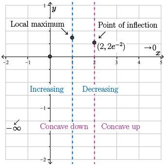
Let's start building our sketch of \(f(x)\). Here we plot the \(y\)-intercept \((0, 0)\) on our graph.
Step 3. Find all discontinuities.
Since \(x\) and \(e^{-x}\) are both continuous functions, so is \(f(x)\). Therefore, \(f(x)\) has no discontinuities.
Step 4. Locate the \(x\)-intercept(s).
Since \(e^{-x} \neq 0\), we have \(f(x) = xe^{-x}=0\) if and only if \(x=0\), the \(x\)-intercept of \(f(x)\) is \(x=0\).
There's nothing new to plot here, as our \(x\)-intercept is actually equal to the \(y\)-intercept, which we've already plotted.
Now let's proceed to steps five and six together.
Steps 5 and 6. Locate the horizontal and oblique asymptotes.
We need to examine the behaviour of the function \(f(x)\) as \(x\) approaches \(\pm\infty\):
Consider \(\displaystyle \lim_{x \rightarrow \infty} xe^{-x} = \lim_{x \rightarrow \infty} \dfrac{x}{e^{x}}\).
Notice that, because \(e\) has a negative exponent, we can rewrite this as a quotient, and consider \(\displaystyle \lim_{x \rightarrow \infty} \dfrac{x}{e^{x}}\). As \(x \to\infty\), the numerator \(x\), of course, approaches infinity as well, and the denominator approaches infinity.
Since this is an indeterminate form of type \(\frac{\infty}{\infty}\), we can use l'Hospital's rule to evaluate the limit:
\[\begin{align*} \lim_{x \rightarrow \infty} xe^{-x} & = \lim_{x \rightarrow \infty} \frac{x}{e^{x}} \\ & = \lim_{x \rightarrow \infty} \frac{\dfrac{d}{dx}\Big(x\Big)}{\dfrac{d}{dx}\Big(e^{x}\Big)} \\ & = \lim_{x \rightarrow \infty} \frac{1}{e^{x}} \\ & = 0 \end{align*}\]
Since the numerator is a constant and the denominator is an exponential that goes to infinity, this limit is equal to zero.
Now consider \(\displaystyle \lim_{x \rightarrow -\infty} xe^{-x}\).
Of course, the term \(x\) approaches negative infinity.
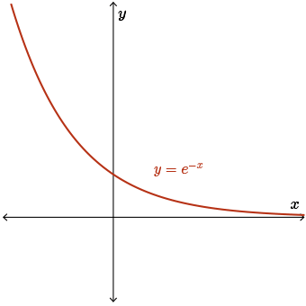
We can see from a sketch of \(y = e^{-x}\) that, as \(x \rightarrow -\infty\), \(e^{-x} \rightarrow \infty\).
Therefore, as \(x\) approaches negative infinity, \(f(x)\) is a very large negative number times a very large positive number, so the product is a very large negative number.
\[ \lim_{x \rightarrow -\infty} x e^{-x} \rightarrow -\infty\]
Let's record this behavior on our graph.
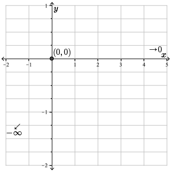
Since \(f(x) =xe^{-x} \geq 0\) for \(x \geq 0\), the function approaches the horizontal asymptote \(y=0\) from above.
Here, we have no oblique asymptote as the function decreases exponentially as \(x \rightarrow -\infty\).
Step 7. Find the critical point(s) of the function (where \(f' = 0\) or DNE).
Since \(f(x)\) is a product, using the product rule, we get
\[\begin{align*} f'(x) & = x\left(\dfrac{d}{dx}\Big(e^{-x}\Big)\right) + e^{-x}\left(\dfrac{d}{dx}\Big(x\Big)\right) \\ & = x (-e^{-x}) + e^{-x}(1) \\ & = e^{-x} - xe^{-x} \\ & = (1-x)e^{-x} \end{align*}\]
Here we have a polynomial times an exponential, so \(f'(x)\) is defined for all real numbers \(x\). Therefore, critical points only occur when \(f'(x)=0\).
Now, \(f'(x)=0\) if one or the other or both of the terms in the product are equal to zero.
As \(e^{-x} \neq 0\), we have \(f'(x)=0\) if and only if \(x=1\).
So \(f\) has exactly one critical point at \(x=1\).
Step 8. Use the critical point(s) to find the intervals of increase/decrease.
The derivative of \(f\) can change signs only at the critical point \(x=1\). So we examine the sign of the derivative on the interval \(x \lt 1\) and the interval \(x \gt 1\). Again, \(f'(x)\) is a product of two factors. The exponential factor is always positive, but the linear factor will change sign.
If \(x \lt 1\), then the factor \(1-x\) is a positive number. If \(x \gt 1\), then the factor \(1-x\) is a negative number. Therefore, the derivative is positive on the interval \(x \lt 1\), and negative on the interval \(x \gt 1\). It follows that the function is increasing on the interval \(x \lt 1\), and decreasing on the interval \(x \gt 1\).
This analysis of the intervals of increase and decrease is summarized in the following table:
| Interval |
\(x\lt 1\) |
\(x \gt 1\) |
| \(f'(x) =(1-x)e^{-x}\) |
\((+)(+)\gt 0\) |
\((-)(+)\lt 0\) |
| \(f(x)\) |
Increasing |
Decreasing |
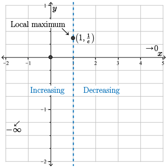
Since the slope is going from positive to negative, we conclude that \(x=1\) is a local maximum, and the maximum value is \(f(1) = 1 e^{-1} = \frac{1}{e} \approx 0.37\).
Let's plot the local maximum, \(\left(1, \frac{1}{e}\right)\), and label the intervals of increase and decrease on our graph.
Step 9. Find the possible point(s) of inflection (where \(f'' = 0\) or DNE).
That is, we find all points at which \(f(x)\) may change concavity. A concavity change may occur where \(f''(x) = 0\) or where \(f''(x)\) does not exist.
We have \(f'(x) = (1-x)e^{-x}= e^{-x}-xe^{-x}\) and so, using the product rule, we have
\[\begin{align*} f''(x) & = \dfrac{d}{dx}\Big(e^{-x}\Big) - \dfrac{d}{dx}\Big(x e^{-x}\Big) \\ & = -e^{-x} -\Bigr[x (-e^{-x}) +e^{-x}\Bigr] \\ & = -2e^{-x} + x e^{-x} \\ & = (x-2)e^{-x} \end{align*}\]
Therefore, \(f''(x) = 0\) if and only if \(x=2\). Note that \(f''(x)\) is defined for all \(x\).
The function value at this point is \(f(2) = 2e^{-2} \approx 0.27\).
Step 10. Find all of the intervals of concavity.
We can now determine the intervals on which the function is concave up and concave down.
Since the domain of \(f''(x)\) is all of \(\mathbb{R}\), the concavity of \(f(x)\) can only change at the point of inflection \(x=2\).
Again, the second derivative is a product of two functions. The second function, the exponential, is always positive. And so the sign is determined by the linear factor \(x-2\).
If \(x \lt 2\), then this factor is negative. If \(x \gt 2\), then this factor is positive. Therefore, the second derivative is negative on the interval \(x \lt 2\), and positive on the interval \(x \gt 2\). So our function is concave down on the first interval, and concave up on the second interval.
Therefore, \(f(x)\) has a point of inflection at \((2,2e^{-2})\).
This analysis of the intervals of concavity is summarized in the following table:
| Interval |
\(x\lt 2\) |
\(x \gt 2\) |
| \(f''(x)=(x-2)e^{-x}\) |
\((-)(+)\lt 0\) |
\((+)(+)\gt 0\) |
| \(f(x)\) |
Concave down |
Concave up |
Let's label these intervals of concavity, along with our point of inflection.
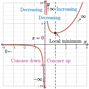
Step 11. Use all of this information to sketch the function.
We make the following sketch.
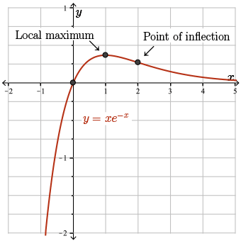
Starting at \((0, 0)\) and using the information recorded on our graph, we see that \(f\) is increasing from \(x=0\) to \(x=1\), and is also concave down.
From \(x=1\) to \(x=2\), it is still concave down, but it switches to decreasing at our local maximum, \(x = 1\).
From \(x=2\) onwards, we still have a decreasing function, but the function switches to concave up at the point of inflection \(x=2\). Here, we see that the function indeed approaches the horizontal asymptote of \(y = 0\) from above.
Finally, on the interval \(x \le 0\), we know our function approaches negative infinity. How fast does it approach negative infinity? Well, we can always plot a few points to help us make this graph if necessary.
Lesson Part 2
Examples
Example 2
Sketch the graph of the function \(y = \dfrac{\cos{(x)}}{1+\sin{(x)}}\).
Solution
Let \(f(x) = \dfrac{\cos{(x)}}{1+\sin{(x)}}\).
Since \(\cos{(x)}\) and \(1+\sin{(x)}\) have period \(2\pi\), so does \(f(x)\).
We will sketch the curve \(y=f(x)\) over the interval \([0,2\pi]\).
Step 1. The functions \(\cos{(x)}\) and \(1+\sin{(x)}\) are both continuous, and so the domain of \(f(x)\) is all real numbers \(x\) such that \(1+\sin{(x)}\neq 0\).
Thus, the denominator is \(0\) when \(\sin(x)=-1\).
We have \(\sin{(x)} = -1\) when \(x = \dfrac{3\pi}{2} + 2k\pi\), for any integer \(k\), and so the domain of \(f(x)\) is
\[\left\{x \in \mathbb{R} : x \neq \frac{3\pi}{2} + 2k\pi, k \text{ is any integer}\right\}\]
On the interval \([0,2\pi]\), \(f(x)\) is only undefined at the point \(x = \dfrac{3\pi}{2}\).
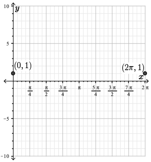
Step 2. The \(y\)-intercept of \(f(x)\) is
\(f(0) = \dfrac{\cos{(0)}}{1+\sin{(0)}} = \dfrac{1}{1+0} = 1\)
Since \(f(x)\) has period \(2\pi\), we also have \(f(2 \pi) = 1\).
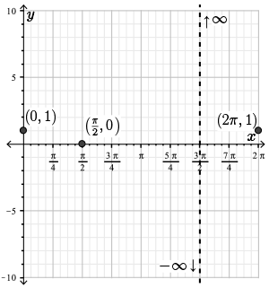
Let's plot these two points, \((0, 1)\) and \((2 \pi, 1)\), on a graph.
Step 3. The function \(f(x)\) has a discontinuity at each point where the denominator is \(0\); in other words, when \(\sin{(x)}=-1\). As we previously mentioned, this occurs when \(x = \dfrac{3\pi}{2} + 2k\pi\) for any integer \(k\).
There is one point of discontinuity in the interval \([0,2\pi]\) at \(x = \dfrac{3\pi}{2}\).
Let's examine the behaviour of the function as it approaches this discontinuity from the left and from the right.
As \(\cos{\left(\dfrac{3\pi}{2}\right)} = 0\) and \(1+ \sin{\left(\dfrac{3\pi}{2}\right)} = 1+(-1) = 0\), the limits as \(x \rightarrow \dfrac{3\pi}{2}^{-}\) and \(x \rightarrow \dfrac{3\pi}{2}^{+}\) are indeterminate forms of type \(\dfrac{0}{0}\).
Therefore, we'll need l'Hopital's rule to compute this limit. Let's start with the limit from the left.
Using L'Hospital's rule we have
\[\begin{align*} \lim_{x \rightarrow \frac{3\pi}{2}^{-} } \dfrac{\cos{(x)}}{1+\sin{(x)}} & = \lim_{x \rightarrow \frac{3\pi}{2}^{-}} \frac{\dfrac{d}{dx}\Big(\cos{(x)}\Big)}{\dfrac{d}{dx}\Big(1 + \sin{(x)}\Big)} \\ & = \lim_{x \rightarrow \frac{3\pi}{2}^{-} } \dfrac{-\sin{(x)}}{\cos{(x)}} \end{align*}\]
provided that the second limit exists or approaches \(\pm \infty\).
As \(x \rightarrow \dfrac{3\pi}{2}^{-}\), the function \(\sin{(x)}\) approaches \(-1\). Therefore, the numerator approaches positive \(1\). The cosine function in the denominator approaches \(0\). And if you look of the graph of \(\cos(x)\), it approaches \(0\) from below. So as \(x \rightarrow \dfrac{3\pi}{2}^{-}\), \(f(x)\) looks like \(1\) over a very small negative number, and so this function goes to negative infinity.
In other words, as \(x \rightarrow \dfrac{3\pi}{2}^{-}\), \(\dfrac{-\sin{(x)}}{\cos{(x)}} \approx \dfrac{-(-1)}{0^{-}} \rightarrow - \infty\) and so
\[\lim_{x \rightarrow \frac{3\pi}{2}^{-}}\dfrac{\cos{(x)}}{1+\sin{(x)}} \rightarrow - \infty\]
Similarly, we can use l'Hopital's rule for the right-hand limit. Again, the limit as \(x \rightarrow \dfrac{3\pi}{2}^{+}\) is equal to the limit of the derivatives.
\[\lim_{x \rightarrow \frac{3\pi}{2}^{+} } \frac{\cos{(x)}}{1+\sin{(x)}} = \lim_{x \rightarrow \frac{3\pi}{2}^{+} } \frac{-\sin{(x)}}{\cos{(x)}}\]
Here, as \(x \rightarrow \dfrac{3\pi}{2}^{+}\), again, \(\sin(x)\) approaches \(-1\). So the numerator approaches \(1\). And the denominator, \(\cos(x)\), again approaches \(0\), but this time, from above. Therefore, we have \(1\), a constant, over a very small positive number. So this function approaches positive infinity.
In other words, as \(x \rightarrow \dfrac{3\pi}{2}^{+}\), we have \(\dfrac{-\sin{(x)}}{\cos{(x)}} \approx\dfrac{-(-1)}{0^{+}} \rightarrow +\infty\) and hence the limit is \(+ \infty\).
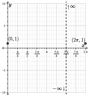
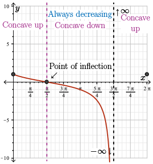
Therefore, \(f(x)\) has a vertical asymptote at \(x= \dfrac{3\pi}{2}\). Approaching this vertical asymptote from the right, \(f(x)\) approaches positive infinity. And approaching this vertical asymptote from the left, our function \(f(x)\) approaches negative infinity. Here we record this information on the graph.
Step 4. The roots of \(f(x)\) occur when the numerator of \(f(x)\) is \(0\), but the denominator is non-zero.
Over the interval \([0,2\pi]\), we have \(\cos{(x)} = 0\) when \(x = \dfrac{\pi}{2}\) and \(x = \dfrac{3\pi}{2}\).
Since
\[\begin{eqnarray*}\sin\left(\dfrac{3\pi}{2}\right)= -1 & \Rightarrow & 1+ \sin\left(\dfrac{3\pi}{2}\right) =0 \\ \sin\left(\dfrac{\pi}{2}\right) = 0 & \Rightarrow & 1 + \sin\left(\dfrac{\pi}{2}\right) \neq 0 \end{eqnarray*}\]
only \(x=\dfrac{\pi}{2}\) is a root of \(f(x)\).
So in the interval \([0,2\pi]\), we have one \(x\)-intercept at \(x = \dfrac{\pi}{2}\).
Here we plot the \(x\)-intercept \((\dfrac{\pi}{2}, 0)\).
Steps 5 and 6. As \(f(x)\) is periodic, the limit of \(f(x)\) as \(x\) approaches positive or negative infinity does not exist.
Step 7. Now let's find the critical points of \(f\).
We find \(f'(x)\) using the quotient rule:
\[\begin{align*} f'(x) & = \dfrac{(1+\sin{(x)}) \dfrac{d}{dx}\Big[\cos{(x)}\Big] - \cos{(x)}\dfrac{d}{dx}\Big[1 + \sin{(x)}\Big]}{(1 + \sin{(x)})^{2}} \\ & = \dfrac{(1+\sin{(x)}) [-\sin{(x)}] - \cos{(x)}[\cos{(x)}]}{(1 + \sin{(x)})^{2}} \\ & = \dfrac{-\sin{(x)} - \sin^{2}{(x)} - \cos^{2}{(x)}}{(1 + \sin{(x)})^{2}} \\ & = \dfrac{-\sin{(x)} - (\sin^{2}{(x)} +\cos^{2}{(x)})}{(1 + \sin{(x)})^{2}} \\ & = \dfrac{-\sin{(x)} - 1}{(1 + \sin{(x)})^{2}} \\ & = \dfrac{-(1+\sin{(x)})}{(1 + \sin{(x)})^{2}} \\ & = -\dfrac{1}{1 + \sin{(x)}} \end{align*}\]
Notice from the formula of \(f'(x)\), we can never have \(f'(x)=0\). And so any critical points of the function must occur when \(f'(x)\) is undefined.
The derivative \(f'(x)\) is undefined when \(\sin{(x)}=-1\), which would make the denominator \(0\).
Over the interval \([0,2\pi]\), this occurs at \(x = \dfrac{3\pi}{2}\).
Although \(f'(x)\) is not defined at \(x=\dfrac{3\pi}{2}\), there is no critical point here since \(x=\dfrac{3\pi}{2}\) does not lie in the domain of \(f\). Recall that we have a vertical asymptote there, although we will need to consider the number \(x=\dfrac{3\pi}{2}\) in the next step when we determine the intervals of increase and decrease.
In particular, since \(f(x)\) has no critical points, the function \(f(x)\) has no local extremes.
Step 8. Now, we find the intervals of increase and decrease.
Since \( \sin{(x)} \geq -1\), by adding \(1\) to both sides of this inequality we have \( 1 + \sin{(x)}\geq 0\) for all \(x\) and, in particular, \(1 + \sin{(x)}\gt 0\) for all \(x\) in the domain of \(f(x)\).
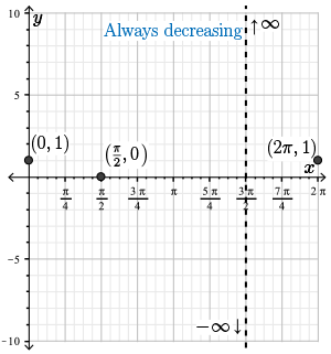
Therefore, we have \(f'(x) = - \dfrac{1}{1+\sin{(x)}} \lt 0 \) for all \(x\) in the domain of \(f(x)\) and so the function \(f(x)\) is always decreasing.
Let's record this information on our graph.
Step 9. Finally, we find all points at which \(f(x)\) may change concavity. A concavity change may occur where \(f''(x) = 0\) or where \(f''(x)\) does not exist. Since \(f'(x) = -\frac{1}{1+ \sin{(x)}} = - (1+\sin{(x)})^{-1}\)
we will use the power rule and the chain rule to find \(f''(x)\):
\[\begin{align*} f''(x) & = +(1 + \sin{(x)})^{-2} \dfrac{d}{dx}\Big[1+\sin{(x)}\Big] \\ & = \dfrac{\cos{(x)}}{(1+\sin{(x)})^{2}} \end{align*}\]
We have \(f''(x) = 0\) when \(\cos(x) = 0\) and \(1 + \sin(x) \neq 0\). This occurs when \(x = \dfrac{\pi}{2}\). We have \(f''\) undefined when \(1 + \sin(x) = 0\).
This occurs when \(x = \dfrac{3\pi}{2}\). These are the only two \(x\) values at which \(f(x)\) may change concavity.
Notice that the only possible point of inflection, \(\left( \frac{\pi}{2} , 0 \right)\), has already been plotted on our graph.
Step 10. We can now determine the intervals on which the function is concave up and concave down.
Again, we will restrict ourselves to the interval \([0,2\pi]\).
The concavity of \(f(x)\) can change either at the point \(x = \frac{\pi}{2}\), or at the discontinuity \(x = \frac{3\pi}{2}\). We will examine the sign of the second derivative \(f''(x)= \dfrac{\cos{(x)}}{(1+\sin{(x)})^{2}}\) on these intervals.
First, we notice that we have a square in the denominator, and so this term is always positive. So the sign of the second derivative will depend on the sign of the numerator, or the cosine function.
Over the interval from \(0\) to \(\frac{\pi}{2}\), \(\cos(x)\) is positive, and so the second derivative is positive.
Between \(\frac{\pi}{2}\) and \(\frac{3\pi}{2}\), \(\cos(x)\) is negative, and so the second derivative is negative.
From \(\frac{3\pi}{2}\) to \(2\pi\), \(\cos(x)\) is positive again, and so the second derivative is positive.
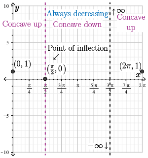
This corresponds to concave up, concave down, and concave up, respectively, as summarized in the following table.
| Interval |
\(0 \lt x \lt \frac{\pi}{2}\) |
\(\frac{\pi}{2} \lt x \lt \frac{3\pi}{2}\) |
\(\frac{3\pi}{2} \lt x\lt 2\pi\) |
| \(f''(x)=\dfrac{\cos{(x)}}{(1+\sin{(x)})^{2}}\) |
\(\dfrac{(+)}{~(+)~} \gt 0\) |
\(\dfrac{(-)}{~(+)~} \lt 0\) |
\( \dfrac{(+)}{~(+)~} \gt 0\) |
| \(f(x)\) |
Concave up |
Concave down |
Concave up |
Observe that \(f(x)\) has a point of inflection at \(x = \dfrac{\pi}{2}\).
Let's record this information, along with the point of inflection, on our graph.
Step 11. Using all of the information that we have gathered, we make the following sketch.
First recall that the function is always decreasing. From \(0\) to \(\frac{\pi}{2}\), the function is concave up, so we draw the following curve.
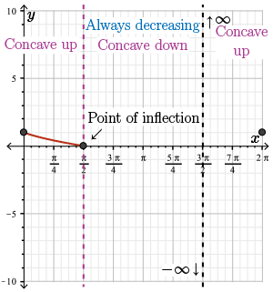
At the point of inflection \(x=\frac{\pi}{2}\), the function becomes concave down and approaches negative infinity as \(x\) approaches the vertical asymptote \(\frac{3\pi}{2}\). So we get the following sketch.
As \(x\) approaches the asymptote from the right, the function \(f(x)\) approaches infinity. And over this interval, it is concave up.
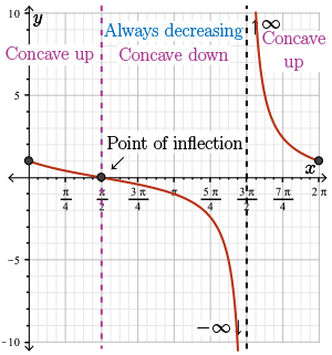
Here we have the final graph of our curve over the interval from \(0\) to \(2 \pi\).
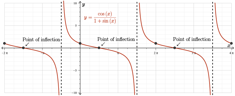
This graph will repeat with period \(2\pi\) and so we get the graph of \(\color{BrickRed}f(x)\).
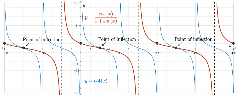
Note the similarities and differences between this graph and the graph of \(\color{NavyBlue}\cot{(x)} = \dfrac{\cos{(x)}}{\sin{(x)}}\). Slightly different, this equation is very similar to the equation of our curve.
Lesson Part 3
Examples
Example 3
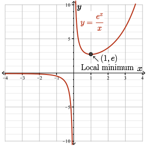
Sketch the graph of the curve \(y = \dfrac{e^{x}}{x}\).
Solution
Let \(f(x) = \dfrac{e^{x}}{x}\).
Step 1. The function \(f(x)\) is a quotient of an exponential and a polynomial both having domain \(\mathbb{R}\).
The function \(f(x)\) is undefined only when the denominator is \(0\) and so the domain of \(f(x)\) is all real numbers except \(x =0\).
Step 2. Since \(f(0)\) is undefined (as we found in step 1), \(f(x)\) has no \(y\)-intercept.
That is, \(f(x)\) does not cross the \(y\)-axis.
Step 3 (discontinuities): Since \(e^{x}\) and \(x\) are both continuous functions, \(f(x)\) is continuous at every point in its domain.
There is only \(1\) discontinuity, occurring at \(x=0\).
Let's examine the behaviour of \(f(x)\) as \(x\) approaches \(0\) from the left and from the right.
As \(x \rightarrow 0^{+}\), \(f(x) = \dfrac{e^{x}}{x} \approx \dfrac{1}{0^{+}} \rightarrow +\infty\).
As \(x \rightarrow 0^{-}\), \(f(x) = \dfrac{e^{x}}{x} \approx \dfrac{1}{0^{-}} \rightarrow -\infty\).
Therefore, \(f(x)\) has a vertical asymptote at \(x=0\).
Let's record this information on a graph.
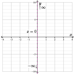
Step 4. Since \(e^x\) is always non-zero, we have \(f(x) \neq 0\) for all \(x\) in the domain of \(f(x)\) and so \(f(x)\) has no \(x\)-intercept.
Steps 5 and 6. We need to examine the behaviour of the function as \(x\) approaches \(\pm\infty\):
\[ \begin{align*} &\displaystyle \lim_{x \rightarrow \infty} \frac{e^{x}}{x} &\text{indeterminant form } \left( \dfrac{\infty}{\infty}\right) \\ & =\displaystyle \lim_{x \rightarrow \infty} \frac{\dfrac{d}{dx}\Big(e^{x}\Big)}{\dfrac{d}{dx}\Big(x\Big)} & \text{by l'Hospital's rule} \\ &=\displaystyle \lim_{x \rightarrow \infty} \frac{e^{x}}{1} \\ &\rightarrow \infty \end{align*} \]
We do not need L'Hospital's rule to examine the limit as \(x\) approaches \(-\infty\). As \(x \rightarrow -\infty\), \(\dfrac{e^{x}}{x} \approx \dfrac{0^{+}}{-\infty} \rightarrow 0\)
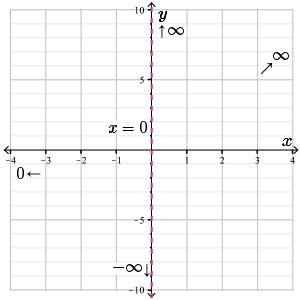
Since \(f(x) \lt 0\) for \(x \lt 0\), the function approaches the horizontal asymptote \(y=0\) from below.
Here, we have no oblique asymptote as the function increases exponentially as \(x \rightarrow \infty\).
Step 7. Next, we determine the critical points of \(f(x)\) to locate the extreme values.
Using the quotient rule, we get
\[f'(x) = \frac{xe^{x} - e^{x}}{x^{2}} = \frac{e^{x}(x-1)}{x^{2}}\]
Since \(e^{x}\) and \(x^{2}\) are positive for all \(x \neq 0\), we have \(f'(x) = 0\) if and only if the term \(x - 1 = 0\). In other words, if \(x=1\).
Therefore, \(f(x)\) has a local extreme at \(x=1\).
Since \(f(x)\) (and \(f'(x)\)) is undefined at \(x=0\), we also have a critical point at \(x=0\).
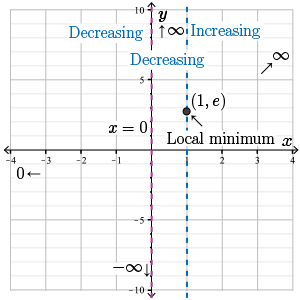
Step 8. Let's examine the sign of the derivative on the intervals \(x\lt 0\), \(0\lt x\lt 1\) and \(x\gt 1\), determined by the critical points of \(f(x)\).
Remember, \(f(x)\) is a quotient where in the numerator we have a product of two terms. As we've noted, \(e^x\) and \(x^2\) are always positive, so the sign of the derivative will depend on the sign of \(x - 1\).
- If \(x\lt 0\), then this term is negative and so the derivative is negative.
- If \(0\lt x\lt 1\), then, again, the term is negative and so the derivative is negative.
- If \(x\gt 1\), then this term becomes positive, and so the derivative is positive.
So the intervals are decreasing, decreasing, and increasing, respectively.
This is summarized as follows:
| Interval |
\(x \lt 0\) |
\(0 \lt x \lt 1\) |
\(x \gt 1\) |
| \(f'(x)=\dfrac{e^{x}(x-1)}{x^{2}}\) |
\(\dfrac{(+)(-)}{~(+)~} \lt 0 \) |
\( \dfrac{(+)(-)}{~(+)~} \lt 0\) |
\(\dfrac{(+)(+)}{~(+)~} \gt 0\) |
| \(f(x)\) |
Decreasing |
Decreasing |
Increasing |
Therefore, since the slope changes from negative to positive at \(x = 1\), there is a local minimum at \(x=1\) with value \(f(1) = \dfrac{e^{1}}{1} = e \approx 2.7\).
Let's record this local minimum and the intervals of increase and decrease on our graph.
Step 9. Finally, we find all points at which \(f(x)\) may change concavity. A concavity change may occur where \(f''(x) = 0\) or where \(f''(x)\) does not exist.
Since \(f'(x) = \dfrac{e^{x}(x-1)}{x^{2}}= \dfrac{xe^{x}-e^{x}}{x^{2}} \) we find \(f''(x)\) using the quotient rule as follows:
\[ \begin{align*} f''(x) & = \dfrac{x^{2} \dfrac{d}{dx}\Bigr[xe^{x}-e^{x}\Bigr] - (xe^{x}-e^{x}) \dfrac{d}{dx} \Bigr[x^{2}\Bigr]}{(x^{2})^{2}} \\ & = \dfrac{x^{2}\Bigr[xe^{x} + e^{x} - e^{x}\Bigr] - (xe^{x} - e^{x})(2x)}{x^{4}} \\ & = \dfrac{x^{3}e^{x} - 2x^{2}e^{x} + 2xe^{x}}{x^{4}} \\ & = \dfrac{e^{x}(x^{2} - 2x + 2)}{x^{3}} \end{align*} \]
Since \(e^{x}\) and \(x^{3}\) are both non-zero for all \(x\) in the domain of \(f(x)\), we have \(f''(x) = 0\) only if \(x^{2}-2x+2=0\).
Using the quadratic formula, we solve this equation and find
\[x = \frac{2 \pm \sqrt{(-2)^{2} - 4(1)(2)}}{2(1)} = \frac{2 \pm \sqrt{-4}}{2}\]
and so this quadratic has no real roots (since we have a negative under the square root).
Therefore, we have \(f''(x) \neq 0\) for all \(x\) in the domain of \(f(x)\).
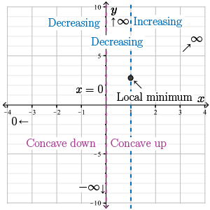
Step 10. We can now determine the intervals on which the function is concave up and concave down.
Since \(f(x)\) has no points of inflection, the only place where the concavity of \(f(x)\) can change is at the discontinuity \(x=0\). Examining the sign of \(f''(x)\) on the intervals \(x\lt 0\) and \(x\gt 0\) gives
| Interval |
\(x \lt 0\) |
\(x \gt 0\) |
| \(f''(x)= \dfrac{e^{x}(x^{2} - 2x + 2)}{x^{3}}\) |
\(f''(-1) = \dfrac{(+)(+)}{(-)} \lt 0\) |
\(f''(1)= \dfrac{(+)(+)}{(+)} \gt 0\) |
| \(f(x)\) |
Concave down |
Concave up |
Let's record this information on the graph.
Step 11. Using all of the information that we have gathered, we make the following sketch.
On the interval \(x \le 0\), we have a decreasing function that's concave down. The function approaches the horizontal asymptote \(y = 0\) from below as \(x \rightarrow -\infty\), and as \(x\) approaches the vertical asymptote \(x = 0\), \(f(x) \rightarrow -\infty\).
For \(x \gt 0\), the function is always concave up but switches from decreasing to increasing at the local minimum of \(x = 1\). As \(x\) approaches the vertical asymptote of \(x = 0\) from the right, the function approaches \(\infty\). And as \(x \rightarrow \infty\), \(f(x) \rightarrow \infty\) as well.
Lesson Part 4
Examples
Challenge Question
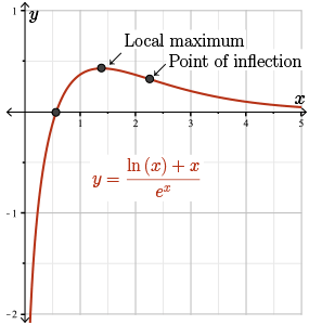
Sketch the graph of the curve \(y = \dfrac{ \ln{(x)}+x}{e^{x}}\).
Solution
We will need to use tools from many different modules to complete this exercise.
Let \(f(x) = \dfrac{ \ln{(x)}+x}{e^{x}}\).
Step 1. Since the domain of \(\ln{(x)}\) is \(x \gt 0\), the domain of \(\ln{(x)} + x\) is \(x \gt 0\).
Since the domain of \(e^{x}\) is \(\mathbb{R}\) and \(e^{x} \neq 0\), the domain of \(f(x)\) is also \(x \gt 0\).
Step 2. Since \(f(0)\) is not defined, the function \(f(x)\) has no \(y\)-intercept.
Step 3.We find the discontinuities. Since \(\ln{(x)}\), \(x\) and \(e^{x}\) are continuous over the entire domain of \(f(x)\), precisely for all \(x \gt 0\) and \(e^{x} \neq 0\), the function \(f(x)\) is continuous at every point in its domain.
We need to examine the behaviour of \(f(x)\) as \(x\) approaches the endpoint \(x=0\) from the right.
As \(x \rightarrow 0^{+}\), we have \(\ln{(x)} + x \rightarrow -\infty\) (because the term \(x\) approaches \(0\) and \(\ln{(x)}\) approaches negative infinity) and \(e^{x} \rightarrow 1\) and so the numerator approaches negative infinity and the denominator approaches a constant of \(1\) which gives
\(f(x) = \dfrac{\ln{(x)}+x}{e^{x}} \rightarrow - \infty\) as \(x \rightarrow 0^{+}\)
Therefore, \(f(x)\) has a vertical asymptote at \(x=0\).
We record this information on our graph.
Step 4. Find the \(x\)-intercept or intercepts of \(f(x)\), provided they exist. Since \(e^{x} \gt 0\) for all \(x\), we have \(f(x) = \dfrac{\ln{(x)}+x}{e^{x}} = 0\) exactly when \(\ln{(x)}+x=0\).
How many roots does this equation have and how do we locate the roots?
Note that the roots of this equation are the points \(x\) that satisfy \(\ln{(x)} = -x\).
So we can draw a sketch of the log function and the line \(y = -x\) to find where they intersect.
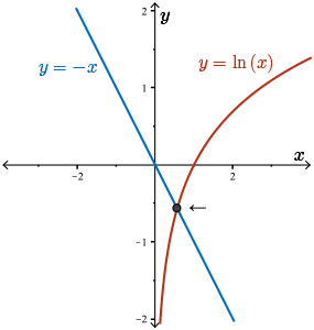
From a sketch of the two functions in question, we conclude that there is exactly \(1\) root, and that the root lies in the interval \([0,1]\).
Here, we can't get an exact value for the root, so we will use Newton's method to approximate the root to \(2\) decimal places, which should be sufficient for our sketch of \(f(x)\).
Using \(g(x) = \ln(x)+x\) and \(x_{1} =1\), try Newton's method now.
Newton's method with \(g(x) = \ln{(x)}+x\), \(g'(x)= \frac{1}{x} + 1\) and \(x_{1}=1\) produces the sequence
\[x_{1} = 1, \ x_{2} = 0.500, \ x_{3} \approx 0.564, \ x_{4} \approx 0.567, \ x_{5} \approx 0.567, \ldots\]
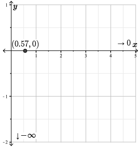
Here we see that the sequence has settled to three decimal places, so we conclude that the root of \(\ln{(x)}+x =0\), and hence the root of \(f(x) = 0\), occurs at \(x \approx 0.57\).
Let's plot this x-intercept on our graph.

Steps 5 and 6. Next, we need to determine the behaviour of \(f(x) = \dfrac{ \ln{(x)}+x}{e^{x}}\) as \(x\) approaches \(\infty\).
Since \(f(x)\) is only defined for \(x\gt 0\), we do not need to consider the limit as \(x\) approaches \(-\infty\). We already have the behavior as \(x\) approaches the left endpoint of \(x = 0\).
Let's look at the behavior of the numerator, \(\ln{(x)}+x\), first. As \(x \rightarrow \infty\), the function \(\ln(x) \rightarrow \infty\) as well, as does the function \(x\). And so the numerator approaches infinity. Similarly, as \(x \rightarrow \infty\), the function \(e^x\) in the denominator approaches infinity.
Therefore, we have an indeterminate form of type \(\dfrac{\infty}{\infty}\), and so we can use L'Hospital's rule, which means we differentiate both the numerator and the denominator.
We have
\[ \begin{align*} & \displaystyle \lim_{x \rightarrow \infty} \frac{ \ln{(x)}+x}{e^{x}} \qquad &\text{indeterminant form }\left(\dfrac{\infty}{\infty}\right) \\ & =\displaystyle \lim_{x \rightarrow \infty} \frac{\frac{1}{x} + 1}{e^{x}} & \text{indeterminant form }\left(\dfrac{1}{\infty}\right) \\ & =0 \end{align*} \]
using l'Hospital's rule.
Now, let's figure out whether the function approaches the horizontal asymptote from above or below.
Since \(\ln{(x)} + x \gt 0\) for all \(x \geq 1\) and \(e^{x} \gt 0\) for all \(x\), we have a quotient of a positive number over a positive number. Therefore, \(f(x) \gt 0\) for all \(x \geq 1\).
Therefore, the function approaches the horizontal asymptote \(y=0\) from above.
Let's record this information on our graph.
Step 7. Let's find the critical points of \(f(x)\).
Using the quotient rule, we find the derivative of \(f(x)\):
\[\begin{align*}f'(x) & = \frac{e^{x}\left(\frac{1}{x} + 1\right) - (\ln{(x)} + x)e^{x}}{(e^{x})^{2}} \\ & = \frac{e^{x} \left(\frac{1}{x} - \ln{(x)} - x+1\right)}{(e^{x})^{2} } \\ & = \frac{\frac{1}{x} - \ln{(x)} - x+1}{e^{x}} \end{align*}\]
Since the denominator is always positive, we have \(f'(x)=0\) exactly when \(\dfrac{1}{x}-\ln{(x)} - x + 1 =0\) or, equivalently, when
\[ \begin{align*} \ln{(x)} & = \dfrac{1}{x} - x + 1 \\ & = \dfrac{1 - x^{2} + x}{x} \end{align*} \]
Here we provide a quick sketch of the functions \(\ln(x)\) and our rational function \( \dfrac{1 - x^{2} + x}{x}\). Of course, we already know what \(\ln(x)\) looks like, and we could also sketch this rational function using the algorithm for curve sketching, but we'll omit these steps here.
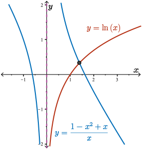
Sketching the function \(\ln{(x)}\) and the rational function \( \dfrac{1 - x^{2} + x}{x}\), we see that the two functions intersect at exactly \(1\) point, and hence there is \(1\) real root of the equation \(f'(x)=0\).
The root is in the interval \([1,2]\). Again, we won't be able to get an exact value for the root, but we use Newton's method with \(g(x) = \dfrac{1}{x}-\ln{(x)} - x + 1 \) to find the root correct to \(2\) decimal places. We'll use technology to do this for us: \(x \approx 1.39\).
Now, this is a bit messy to do by hand using just your personal calculator, but go ahead and give it a go if you like. We do have the tools necessary to compute this. Try this on your own!
Therefore, the root of \(f'(x)=0\) is \(x \approx 1.39\).
Since \(f'(x)\) is defined all points in the domain, for all \(x\gt 0\), the only critical point of \(f(x)\) is \(x\approx 1.39\), which is a local extreme.
Step 8. Next we will examine the sign of the derivative on the intervals \(0\lt x\lt 1.39\) and \(x \gt 1.39\). The sign of the first derivative can change at the critical point that we found in step 7. We'll use our usual table to determine the sign of the first derivative.
| Interval |
\( 0\lt x\lt 1.39\) |
\(x \gt 1.39\) |
| \(f'(x)\) |
\(f'(1) \gt 0\) |
\(f'(2)\lt 0\) |
| \(f(x)\) |
Increasing |
Decreasing |
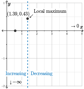
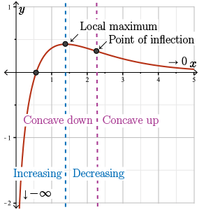
Therefore, the point \(x\approx 1.39\) is a local maximum, and the maximum value is \(f(1.39) \approx 0.43\).
Let's plot the local maximum on our graph and record the information about the intervals of increase and decrease.
Step 9. Finally, we find all points at which \(f(x)\) may change concavity. A concavity change may occur where \(f''(x) = 0\), or were \(f''(x)\) does not exist.
Since \(f'(x) =\dfrac{\frac{1}{x} - \ln{(x)} - x+1}{e^{x}}\), using the quotient rule, we have
\[\begin{align*}f''(x) & = \frac{e^{x}\left(-\frac{1}{x^{2}} - \frac{1}{x}-1\right) - \left(\frac{1}{x} - \ln{(x)} - x +1\right)e^{x}}{(e^{x})^{2}}\\ & = \frac{e^{x} \left(-\frac{1}{x^{2}} - \frac{1}{x}-1 - \frac{1}{x} + \ln{(x)} + x - 1\right)}{(e^{x})^{2}} \\ & = \frac{-\frac{1}{x^{2}}- \frac{2}{x} + \ln{(x)} + x - 2}{e^{x}}\end{align*}\]
The function \(f''(x)\) is defined for all \(x\gt 0\) and \(f''(x) = 0\) if and only if the numerator is \(0\). That is, \(-\frac{1}{x^{2}}- \frac{2}{x} + \ln{(x)} + x - 2 = 0\).
As in Step 7, we can use a sketch of \(\ln{(x)}\) and an appropriate rational function to determine that this equation has exactly \(1\) real root, and we use Newton's method to approximate the root to \(2\) decimal places.
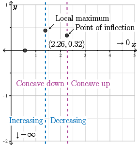
Doing so, we find that \(f(x)\) has one point of inflection at \(f''(x)=0\) when \(x \approx 2.26\).
Now, this application of Newton's method may be a bit much to do with just your personal calculator, but technology can do it for you.
Step 10. Examining the sign of the second derivative on the intervals \(0\lt x\lt 2.26\) and \(x\gt 2.26\), we get the following:
| Interval |
\( 0\lt x\lt 2.26\) |
\(x \gt 2.26\) |
| \(f''(x)\) |
\(f''(2) \lt 0\) |
\(f''(3)\gt 0\) |
| \(f(x)\) |
Concave down |
Concave up |
Let's plot our point of inflection and record the information about the concavity of \(f\).
Step 11. Using all of the information that we have gathered, we make the following sketch.
As we have seen in this module, our algorithm for curve sketching applies nicely to curves involving exponential, logarithmic, and trigonometric functions as well. The only real difference here from back when we were sketching only polynomials and rational functions is that we often require L'Hospital's rule to aid in finding limits, and sometimes even Newton's method to locate roots, critical points, and points of inflection. You'll get a chance to practice this algorithm in the student exercises.
Quiz
See the quiz in the side navigation.