Lesson Part 1

In This Module

• We will learn Newton's method for approximating the roots of an equation of the form \(f(x)=0\).

We know that the quadratic formula will find the exact roots in the case where \(f(x)\) is a quadratic polynomial, but how about the roots of a function like \(f(x) = \sin(x) - x^{2}\) where there is no such formula to calculate the exact roots?

What are the roots of the equation \(f(x) = \sin(x) - x^{2}\)?

The fundamental tool used in this method is the tangent line approximation.

Finding Roots

Question

What are the roots of the equation \(ax^{2} + bx + c = 0\)?

Solution

This equation should look very familiar. We have a well-known quadratic formula that finds the roots of any quadratic equation

\[x = \dfrac{-b \pm \sqrt{b^{2}-4ac}}{2a}\]

There are also formulas for finding the roots of equations involving \(3^{rd}\) and \(4^{th}\)-degree polynomials, although they are much more complicated than the above.

For polynomials that are degree \(5\) and above, there is no such formula.

How might we approximate the roots of such an equation? What if our equation involves functions other than polynomials?

Question

What are the roots of the equation \(\sin(x)-x^{2}=0\)?

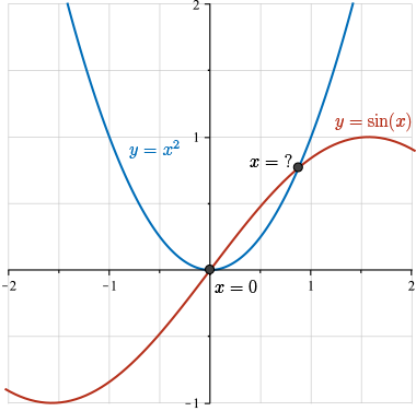
If you graph the curves \(y=\sin(x)\) and \(y=x^{2}\), then you will see that these functions intersect at exactly \(2\) points, and hence there are exactly \(2\) roots of the above equation.

One of these roots is \(x=0\) but what is the value of the other root?

We cannot get an exact answer for the \(2^{nd}\) root of this equation, but we can approximate the root to any degree of accuracy that we would like.

One method to do so is called Newton's method (also called the Newton-Raphson method) and is a relatively straightforward application of tangent line approximation.

Linearization

If there is a tangent line to the curve \(y=f(x)\) at the point \((a,f(a))\), then this tangent line may provide a good approximation of the curve near \(x=a\).

That is, since the curve lies close to this tangent line near the point \((a,f(a))\), this line can be used to approximate the values of the function.

Recall that the equation of the line having slope \(m\) and passing through the point \((x_{1}, y_{1})\) is given by

\[y - y_{1} = m (x-x_{1})\]

The tangent line to \(y=f(x)\) at the point \(x=a\) has slope \(f'(a)\) and passes through the point \((a, f(a))\), and hence the equation of this tangent line is \(y -f(a) = f'(a)(x-a)\) or equivalently

\[y =f(a) + f'(a)(x-a)\]

Of course, this formula holds provided that the tangent line does not have an infinite slope.

If \(f(a)\) and \(f'(a)\) can be readily calculated, then this tangent line can be useful for approximating values of \(f(x)\) for \(x\) near \(a\). So we make the following definition:

The linearization of \(f\) at \(a\) is defined to be the function

\[L(x)=f(a)+f'(a)(x-a)\]

Here, \(L(x)\) is equal to the right-hand side of the tangent line equation. By our earlier comments, we have \(f(x)\approx L(x)\) if \(x\approx a\). This is the idea of using a line to approximate a function. This approximation is called the linear approximation of \(f(x)\) at \(x=a\).

Lesson Part 2

Using Linearization to Approximate Square Roots

Example 1

Use the linearization of \(f(x) = \sqrt{x}\) at \(x=1\) to approximate the value of \(\sqrt{1.1}\).

Solution

We know that if we zoom in enough on the graph of a smooth curve, then the curve is close to a straight line.

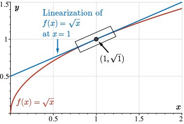
As such, the linearization of \(f(x)\) at \(x=1\) should provide a reasonably good approximation for the values of \(f(x)\) for \(x \approx 1\).

Since \(f(x)= \sqrt{x}\), we have \(f'(x) = \dfrac{1}{2\sqrt{x}}\), so \(f(1) = \sqrt{1} = 1\) and \(f'(1) = \dfrac{1}{2\sqrt{1}} = \dfrac{1}{2}\).

Therefore, the linearization of \(f\) at \(x=1\) is

\[ L(x) = f(1) + f'(1)(x-1) = 1 + \dfrac{1}{2}(x-1)\]

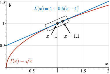
As we can see in the picture, when \(x=1.1\), we have \(L(1.1) \approx f(1.1)\).

This is because the tangent line to \(f(x) = 1\) is very close to the curve as long as you keep the values of \(x\) close to \(x = 1\). In fact, we would have to zoom in pretty close in this picture to see any difference at all between the value of \(L(x)\) and the value of \(f(x) = 1.1\).

Now we use the linearization to approximate \(f(1.1)\) by substituting \(x = 1.1\) into the formula. We can easily calculate

\[L(1.1) = 1+\dfrac{1}{2}(1.1-1)=1.05\]

So, we estimate that

\[\sqrt{1.1} = f(1.1)\approx L(1.1)=1.05\]

That is, the linear approximation of \(\sqrt{1.1}\), which is equal to \(f(1.1)\), is equal to \(1.05\).

So how good is this approximation?

Checking with a calculator, we get \(\sqrt{1.1} \approx 1.0488\ldots\) and so the approximation is correct up to two decimal places.

Now, why is this linearization useful? Well, since the square root of \(1\) is an integer, \(f (1)\) and \(f'(1)\) are both integers and easy to calculate. And so the formula for \(L (x)\) is easy to calculate. It's not so easy to calculate \(f\) of values of \(x\) that are near \(1\), e.g., \(1.1\), \(1.2\), or \(0.9\), \(0.8\). So we use the fact that the square root of \(1\) is easy to compute to approximate more difficult square roots near \(1\).

We could use the linearization of \(\sqrt{x}\) at \(x = 4\) in a similar way to approximate the square roots of numbers that are close to \(4\). What about the square roots of values of \(x\) where \(x\) is not close to a perfect square?

Example 2

Use the linearization of \(f(x)=\sqrt{x}\) at \(x=1\) to approximate the value of \(\sqrt{2}\).

Solution

From the previous example, the linearization of \(f(x)=\sqrt{x}\) at \(x=1\) is given by

\[L(x)=1+\dfrac{1}{2}(x-1)\]

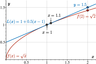
Since \(x=2\) is farther from \(x=1\), we would expect this linearization to give a worse approximation of \(\sqrt{2}\) than it gave for \(\sqrt{1.1}\).

This is apparent in the graph shown.

Here we see again the tangent line to the curve at \(x = 1\) and the curve \(f(x)=\sqrt{x}\). Notice that the tangent line is very close to the curve near \(x = 1.1\), but much farther from the curve around \(x = 2\).

Here, we have

\[L(2)=1+\dfrac{1}{2}(2-1)=1+\dfrac{1}{2}=1.5\]

How good is this approximation? Using a calculator, \(\sqrt{2}\approx 1.414\), so the linear approximation \(\sqrt{2}=f(2)\approx L(2)\) is not correct up to a single decimal place. (Recall that the approximation of \(\sqrt{1.1}=f(1.1) \approx L(1.1)\) was correct up to two decimal places.)

So how do we approximate square roots when the value of x is not close to a perfect square? How do we approximate \(\sqrt{2}\) more accurately?

Lesson Part 3

Newton's Method

Now we're ready to introduce the topic of Newton's method. One application of the method of linearization is Newton's method.

Newton's method can be used to approximate the roots of equations of the form \(f(x)=0\).

In particular, it can be used to approximate the positive root of the equation \(x^2-2=0\) to any degree of accuracy we would like. (This is, of course, equivalent to approximating the value of \(\sqrt{2}\) to any degree of accuracy.)

We will now introduce the theory behind Newton's method, while attempting to approximate the positive root of the equation \(x^2-2=0\) more accurately.

First, we guess that the positive root of the equation \(f(x)=x^2-2=0\) is near \(x=3\).

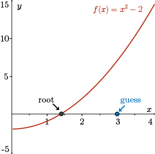
Now, of course, we just discussed how the square root is actually around \(1.4\). Well, let's pretend that we have no analysis or no immediate knowledge of the value of \(\sqrt{2}\). The fact that this initial guess is so far from the exact value will actually show us how powerful Newton's method is.

The next step is to find the linearization of \(f(x)\) at \(x=3\):

\[L(x)=f(3)+f'(3)(x-3)=7+6(x-3)\]

Then, our linear approximation gives us \(f(x)\approx L(x)\) for \(x\approx 3\).

Since \(L(x)\) is our approximation of \(f(x)\), we use the \(x\)-intercept of \(L(x)\) to approximate the \(x\)-intercept of \(f(x)\) (that is, the root of \(f(x)=0\)).

If the root of \(f(x)=0\) is indeed near \(x=3\), then this approximation will be useful.

Here, we see a graphical representation of this process.

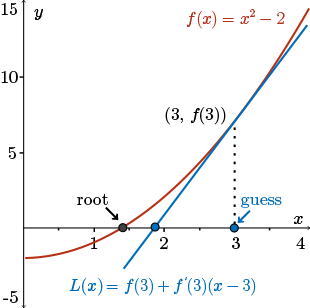
Here we see a graphical representation of this process. Here we have our plotted guess \(x=3\), the tangent line to the curve, or the linearization of \(f (x)\) at \(x= 3\), and the location of the actual root of \(f (x)= 0\). In the picture, it is clear that the \(x\)-intercept of \(L(x)\) is a better approximation to the root of \(f (x)= 0\) than \(x = 3\).

Setting \(L(x)=0\) and solving for the \(x\)-intercept, we get

\[0=7+6(x-3)\implies x-3=-\dfrac{7}{6} \implies x=3-\dfrac{7}{6}=\dfrac{11}{6}\]

We take \(x=\frac{11}{6}\) as our “updated approximation” of the root.

Now, we repeat this process, this time with \(x=\frac{11}{6}\) instead of the original guess of \(x=3\).

To keep track of the process we're developing, we will introduce some notation:

Let \(x_{1} = 3\) denote our first guess, and let \(x_{2} = \dfrac{11}{6}\) denote our second approximation.

Now, we repeat the same process with our new guess \(x_{2}\).

First, we find the linearization of \(f\) at \(x_{2}=\dfrac{11}{6}\).

Evaluating, we have \(f\left(\dfrac{11}{6}\right) = \left(\dfrac{11}{6}\right)^{2} - 2 = \dfrac{121}{36} - 2 = \dfrac{49}{36}\) and \(f'\left(\dfrac{11}{6}\right) = 2 \left(\dfrac{11}{6}\right) = \dfrac{11}{3}\)

Substituting these values into the equation for our tangent line approximation, we get that the linearization is

\[L(x) = f(x_{2}) + f'(x_{2})(x-x_{2}) = \dfrac{49}{36} + \dfrac{11}{3}\left(x-\dfrac{11}{6}\right)\]

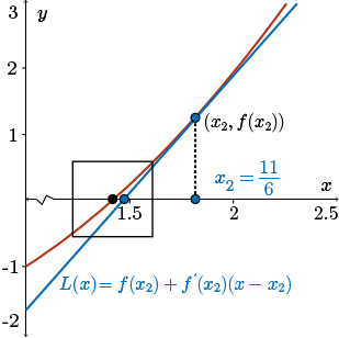
Now, again, look at the picture. We have our new guess \(x_2\), the point \((x_2, f(x_2))\), and the tangent line drawn at that point.

Again, as we see in the picture, the \(x\)-intercept of this new line is even “closer” to the desired root than our second approximation \(x_{2} = \dfrac{11}{6}\).

By setting \(y=0\) and solving for \(x\), we get the \(x\)-intercept:

\[ 0 = \dfrac{49}{36} + \dfrac{11}{3}\left(x-\dfrac{11}{6}\right)\]

Rearranging this equation and multiplying through by \(\dfrac{3}{11}\), we get

\[\begin{align*}\Longrightarrow x-\dfrac{11}{6} & = -\left(\dfrac{49}{36}\right)\left(\dfrac{3}{11} \right) \\ \Longrightarrow x & = \dfrac{11}{6} - \dfrac{49}{132} = \dfrac{193}{132} \end{align*}\]

Hence the \(x\)-intercept is \(\dfrac{193}{132} \approx 1.46\), to two decimal places.

As this guess is even better than \(x_2\), we will make our next approximation \(x_{3} = \dfrac{193}{132}\).

Now, here's a graphical summary of what was happening with our first three approximations. We're generating a sequence of approximations for the root \(x_1\), \(x_2\), \(x_3\), and each one is better than the last.

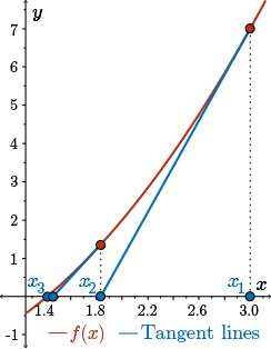
If we repeat this process, then we get the following sequence of numbers. Here we present the exact values, along with their decimal values rounded to three decimal places.

\[\begin{align*} x_{1}&=3 \\ x_{2} &= \dfrac{11}{6} \approx 1.833 \\ x_{3} &= \dfrac{193}{132} \approx 1.462 \\ x_{4} &=\dfrac{72097}{50952} \approx 1.415 \\ x_{5} &= \dfrac{10390190017}{7346972688} \approx 1.414 \end{align*} \]

We got the fractions for \(x_4\) and \(x_5\) using the help of technology.

If we look at the decimal expansion for these fractions and round it to three decimal places, we notice that the \(5^{th}\) approximation, \(x_{5}\), is correct up to at least three decimal places with the number \(\sqrt{2}\).

In fact, if you check on your calculator, \(x_{5}\) agrees with the value of \(\sqrt{2}\) up to six decimal places!

Here we see the decimal expansion of \(x_5\) up to eight decimal places.

\[\begin{align*} x_{5} = \dfrac{10390190017}{7346972688} &=1.41421378 \ldots \\ \sqrt{2} &= 1.41421356\ldots \end{align*}\]

This method for approximating roots of equations is called Newton's method (or the Newton-Raphson method).

Lesson Part 4

Newton's Method

Let's try and formalize this process.

Let's recap this process for finding roots of an equation \(f(x) = 0\). We have the following steps:

1. Make a guess at a root of \(f\) and call this guess \(x_{1}\).

2. Find the tangent line approximation to \(f\), or the linearization of \(f\), at \(x_{1}\):

   \[y = f(x_{1}) + f'(x_{1})(x-x_{1})\]

   Remember, we did so in our example for \(x_1= 3\).

   Next we find the \(x\)-intercept of this line. We do so by setting \(y= 0\) and rearrage to solve for \(x\).

   \[ \begin{align*} 0 & = f(x_{1}) + f'(x_{1})(x-x_{1})\\ \Longrightarrow x-x_{1} & = -\dfrac{f(x_{1})}{f'(x_{1})} \\ \Longrightarrow x & = x_{1} -\dfrac{f(x_{1})}{f'(x_{1})}\end{align*}\]

   So here we have an equation for computing the next guess given the guess of \(x_1\).

3. Let \(x_{2} = x_{1} -\dfrac{f(x_{1})}{f'(x_{1})}\), the \(x\)-intercept found in step 2), and now we repeat the process by returning to step 1) with \(x_{2}\) in place of \(x_{1}\).

Repeating this process, we generate the following sequence of approximations:

\[\begin{align*} x_{1} & = \text{ guess at root} \\ x_{2} & = x_{1} -\dfrac{f(x_{1})}{f'(x_{1})}\\ x_{3} & = x_{2} -\dfrac{f(x_{2})}{f'(x_{2})} \\ x_{4} & = x_{3} -\dfrac{f(x_{3})}{f'(x_{3})} \\ & \vdots\end{align*}\]

In general, if we have the \(n^{th}\) term in the sequence, \(x_n\), we can get the next term, \(x_{n+ 1}\), using the following equation.

Now we have a formula for generating the terms in the sequence using Newton's method without explicitly referring to tangent lines or \(x\)-intercepts. But it's important to remember how we derived this formula, that in fact it did come from this geometric argument. This fact will be important when later on we attempt to predict for which initial guesses will Newton's method be successful.

Under which conditions does Newton's method produce a sequence that converges to a root of \(f(x)=0\)?

Lesson Part 5

Newton's Method

Example 3

Starting with \(x_{1} = 1\), find the \(3^{rd}\) approximation \(x_{3}\) to the positive root of the equation \(x^{2}+x-1=0\). Check the accuracy of the approximation using the quadratic formula.

Solution

Let \(f(x) = x^{2}+x-1\), then by the power rule, we have \(f'(x) = 2x + 1\).

Now let's apply the formula for Newton's method. Computing \(x_2\), we use the following formula:

\[\begin{align*} x_{1} & = 1 \\ x_{2} & = x_{1} - \dfrac{f(x_{1})}{f'(x_{1})}= 1 - \dfrac{f(1)}{f'(1)} = 1- \dfrac{(1)^2+1-1}{2(1)+1} = 1 - \dfrac{1}{3} = \dfrac{2}{3} \end{align*}\]

Simplifying this expression, we get an answer of \(\dfrac{2}{3}\). Therefore, our second approximation is equal to \(\dfrac{2}{3}\).

Finally, we need to find the third approximation, \(x_3\), using the same formula, but with \(x_2\) in place of \(x_1\).

\[ x_{3} =x_2 - \dfrac{f(x_2)}{f'(x_2)}=\dfrac{2}{3} - \dfrac{f\left(\frac{2}{3}\right)}{f'\left(\frac{2}{3}\right)} = \dfrac{2}{3} - \dfrac{\frac{1}{9}}{\frac{7}{3}} = \dfrac{13}{21}\]

Therefore, our third approximation, as asked for in the question, is \(\dfrac{13}{21}\).

Now, since we started with a quadratic equation, we can, of course, find the exact value of this route using the quadratic formula.

Since \(a= 1\), \(b= 1\), and \(c-1\), we have

\[x = \dfrac{-1 \pm \sqrt{1^{2} - 4(1)(-1)}}{2(1)} = \dfrac{-1 \pm \sqrt{5} }{2}\]

Exactly one of these roots is positive, which is the root we're looking for. So the positive root is

\[x = \dfrac{-1+\sqrt{5}}{2} \approx 0.618\]

Using our calculator and rounding to three decimal places, we get that \(x\) is approximately equal to \(0.618\).

If we check out the decimal expansion of \(x_{3} = \dfrac{13}{21} \approx 0.619\), our approximation was correct up to two decimal places.

Now at this point, you should ask yourself, what happens if we start with \(x_{1} = -1\) instead? What about \(x_{1} = 0\)?

Now would be a good time to pause the lesson and work out the third approximation's \(x_3\) for each of these two cases. Are they similar approximations to the case of \(x_1= 1\)? Are they different? How different?

Remarks

For certain functions \(f(x)\) and guesses \(x_{1}\), the sequence of numbers generated by Newton's method \(x_{1}, x_{2} ,x_{3},\ldots\) will converge to a root of the equation \(f(x)=0\) quite quickly (like in the previous examples).

However, in many cases, the sequence may converge very slowly, or not at all.

This is often the case if the tangent line to \(f\) at \(x_{1}\) is close to horizontal.

Can you explain why?

What happens if the equation, \(f(x) = 0\), has more than one root? This was the case in example 1 and example 2. Will different guesses converge to different roots?

Now it's time to explore the given Maple worksheet. Here, you be asked to use Newton's method to attempt to locate roots of various equations. The goal is to think about what types of guesses are successful or unsuccessful. Can you figure out why, geometrically, this might be the case?

Another question to ask is how sensitive is Newton's method to your initial guess. Can initial guesses that are very close together generate vastly different sequences? Try and figure out what happens in the case of multiple roots. Once you finish, come back, and we'll try and summarize this worksheet with a final example.

Investigation

See the investigation in the side navigation.

Lesson Part 6

Newton's Method

Example 4

The equation \(x^{3} - 4x -1 = 0\) has three real roots, exactly one of which is positive. Find the value of the positive root correct to five decimal places.

Solution

Here we have a cubic equation. So naturally, the first thing to do is see if we can factor it. First, we check if the equation has any rational roots.

By the rational roots theorem, the only possible rational roots are \(\pm 1\) and so we check \(f(-1) = (-1)^{3} - 4(-1) - 1 = 2\) and \(f(1) = (1)^{3} - 4(1) - 1 = -4\) neither of which is equal to \(0\). So we conclude that the equation has no rational roots.

Since we cannot factor the cubic polynomial easily, we will use Newton's method to locate the positive root.

Let's generate Newton's formula. Let \(f(x) = x^{3} - 4x - 1\), then \(f'(x) = 3x^{2} - 4\).

Therefore, the formula for Newton's method is given by

\[x_{n+1} = x_{n} - \dfrac{f(x_{n})}{f'(x_{n})} = x_{n} - \dfrac{x_{n}^{3} - 4x_{n} - 1}{3x_{n}^{2} - 4} \]

for all \(n \geq 1\). That is, this formula holds for all approximations past our first guess.

Since we are looking for a positive root, let's start with a positive number as our guess: \(x_{1} = 1\).

Using the formula for Newton's method, we generate the following sequence of approximations:

\[x_{2} = x_{1} - \dfrac{x_{1}^{3} - 4x_{1} - 1}{3x_{1}^{2} - 4} = 1 - \dfrac{(1)^{3} - 4(1) - 1}{3(1)^{2} - 4} = 1 - \dfrac{(-4)}{(-1)} = 1 - 4 = -3\]

So right away, we see something going wrong. If we're looking for a sequence that approaches a positive root, our next approximation has already moved to a negative number. If we continue on and compute \(x_3\) using the same formula, now with \(x_2 = -3\), then we get

\[ \begin{align*} x_{3} & =x_{2} - \dfrac{x_{2}^{3} - 4x_{2} - 1}{3x_{2}^{2} - 4} = -3 - \dfrac{(-3)^{3} - 4(-3) - 1}{3(-3)^{2} - 4} \\ & = -3 - \dfrac{(-16)}{(23)} = -3 + \dfrac{16}{23} \\ & = -\dfrac{53}{23} \approx -2.30435 \end{align*}\]

Okay, so we have another negative number. But it is moving in the positive direction. If we compute \(x_4\), \(x_5\), and \(x_6\), we get the following approximations rounded to five decimal places.

\[\begin{align*} x_{4} & \approx -1.96749 \\ x_{5} & \approx -1.86947 \\ x_{6} & \approx -1.86087 \end{align*}\]

It looks as though this sequence is approaching a number. But the sequence seems to be approaching a number around \(-1.86\), and so we suspect that we have chosen a bad guess \(x_{1}\) for finding the positive root.

In fact, this sequence is approaching one of the negative roots of the equation.

Hopefully, if you looked at the Maple worksheet, you figured out that your best chance for success with Newton's method is to find a guess, \(x_1\), that's as close as possible to the root you're trying to find.

To determine a better initial guess, we need further analysis to narrow down the location of the positive root. Let's do so without trying to graph the function.

If we evaluate the function, \(f\), at various small integer values, \(x=0, 1, 2, 3, \ldots\), we get the following. Hopefully, we'll get lucky and figure out a way to locate the root.

\[\begin{align*} f(0) & = -1\\ f(1) & = -4\\ f(2)& = -1\\ f(3) & = 14 \end{align*}\]

So here we see the function go from a negative value to a positive value.

Since \(f(2)=-1\) is negative and \(f(3) =14\) is positive, we conclude that we must have a root in the interval \([2,3]\). Why can we conclude that?

The continuous polynomial must cross the \(x\)-axis at some point between \(x=2\) and \(x=3\).

Therefore, there must be some number \(a\) in the interval \((2,3)\) such that \(f(a)=0\).

A formal justification of this fact is the content of what is called the intermediate value theorem.

This theorem is generally presented in any university calculus class.

Since \(f(2)=-1\) is much closer to zero than \(f(3)=14\), we suspect that the root may be closer to \(2\) and so we choose \(x_{1} = 2\).

Again, we apply Newton's method. Notice that we do get positive numbers.

\[\begin{align*} x_{1} & =2 \\ x_{2} & =x_{1} - \dfrac{x_{1}^{3} - 4x_{1} - 1}{3x_{1}^{2} - 4} = 2 - \dfrac{(2)^{3} - 4(2) - 1}{3(2)^{2} - 4} = 2 - \dfrac{(-1)}{(8)} = 1+ \dfrac{1}{8} = \dfrac{17}{8} = 2.125 \\ x_{3} & \approx 2.114975450 \\ x_{4} & \approx 2.114907545 \\ x_{5} & \approx 2.114907541 \end{align*}\]

We've expanded the fractions and rounded them to nine decimal places of accuracy. It appears that this sequence is settling down.

Since \(x_{4}\) and \(x_{5}\) agree on (at least) five decimal places, we conclude that the positive root of the equation, to five decimal places of accuracy, is \(x = 2.11491\).

Lesson Part 7

Newton's Method

Example 4

The equation \(x^{3} - 4x -1 = 0\) has three real roots, exactly one of which is positive. Find the value of the positive root correct to five decimal places.

Solution

Why was \(x_{1} = 1\) a bad guess, while \(x_{1} = 2\) was a good guess?

Generally, the best guesses are numbers \(x_{1}\) that are relatively close to the root in question.

What does relatively close mean? That's a little vague. Well, it's vague, because that depends on the function being considered. There's no absolute way of defining how close you need to be to the root to have success.

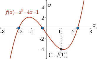
Consider the graph of the cubic \(f(x) = x^{3} - 4x - 1\).

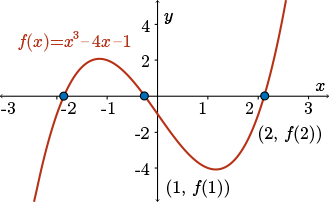
The three roots lie in the intervals \([-2,-1]\), \([-1,0]\), and \([2,3]\).

(Note that we can also locate the intervals in which the two negative roots lie by evaluating the function \(f\) at various negative points \(x=-1,-2,-3,\dots\))

Now, let's discuss briefly what happens if we pick \(x_1\) to be these various interval endpoints.

• If we choose \(x_{1}=-2\) or \(x_{1}=-1\), then the sequence approaches the root in the interval \([-2, -1]\).
• If we choose \(x_{1}=0\), then the sequence approaches the root in the interval \([-1,0]\).
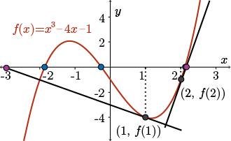
• If we choose \(x_{1} =2\) or \(x_{1} = 3\), then the sequence approaches the positive root.

It looks like within reason, if we pick these endpoints to be our starting guesses, then the generated sequences are converging to roots that are pretty close to the starting point.

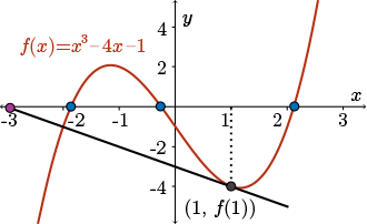
But recall that we had this strange behavior for \(x_1= 1\). Can you see why \(x_{1} = 1\) generated a sequence approaching the root in the interval \([-2,-1]\) instead of the other two roots that are actually closer?

This has everything to do with the fact that the slope of \(f(x)\) around \(x=1\) is close to horizontal. What is the tangent line at that point going to look like, and what is its corresponding \(x\)-intercept. In other words, what \(x_2\) will that generate?

As you can see in the picture, the \(x\)-intercept of the tangent line drawn to \((1, f (1))\) is negative. It moves us from a positive number to a number so negative it's moved past all three roots.

What would happen with other initial guesses \(x_1\). To further examine the sensitivity of Newton's method to the initial guess chosen, we present the following summary.

In this table, we present many initial guesses, \(x_1\) ranging from \(- 1000\) to \(1000\). In the right hand column, you'll see a particular approximation from the sequence. The particular term from the sequence that is given represents the time at which the sequence has stopped changing on the first two decimal places. For example, if we choose \(x_1\) to be equal to \(- 1000\), we see that \(x_{19}\) is equal to \(-1.86\) up to two decimal places. And moreover, \(x_{20}\), \(x_{21}\), and every other term in the sequence will agree with \(x_{19}\) on the first two decimal places.

Now take a second to have a look at this table and see what you notice.

\(x_{1}\)	Correct to two decimal places
\(-1000\)	\(x_{19} = -1.86\ldots\)
\(-100\)	\(x_{14} = -1.86\ldots\)
\(-30\)	\(x_{11} = -1.86\ldots\)
\(-5\)	\(x_{7} = -1.86\ldots\)
\(-3\)	\(x_{5} = -1.86\ldots\)
\(-2\)	\(x_{3} = -1.86\ldots\)
\(-1.2\)	\(x_{8} = -1.86\ldots\)
\(-1.1\)	\(x_{7} = 2.11\ldots\)
\(-1\)	\(x_{7} = -1.86\ldots\)
\(-0.9\)	\(x_{4} = -0.25\ldots\)
\(-0.5\)	\(x_{3} = -0.25\ldots\)
\(0\)	\(x_{2} = -0.25\ldots\)
\(0.5\)	\(x_{4} = -0.25\ldots\)
\(0.8\)	\(x_{7} = -0.25\ldots\)
\(0.9\)	\(x_{5} = -1.86\ldots\)
\(1\)	\(x_{6} = -1.86\ldots\)
\(1.1\)	\(x_{9} = -1.86\ldots\)
\(1.2\)	\(x_{10} = 2.11\ldots\)
\(2\)	\(x_{3} = 2.11\ldots\)
\(3\)	\(x_{5} = 2.11\ldots\)
\(5\)	\(x_{6} = 2.11\ldots\)
\(30\)	\(x_{11} = 2.11\ldots\)
\(100\)	\(x_{14} = 2.11\ldots\)
\(1000\)	\(x_{20}= 2.11\ldots\)

It seems like, within reason, if we pick \(x_1\) to be around the point \(- 1.86\), then our sequence converges to \(- 1.86\). Similarly for numbers around \(- 0.25\), they seem to converge for the most part to the root \(- 0.25\). And the same thing holds for the root \(2.11\).

Now, you'll see that there's two problems with this pattern. At \(- 1.1\), which is relatively close to \(- 1.86\), we have this sequence converging to the root \(2.11\). And then we go back at \(- 1\) to converging to \(- 1.86\) again.

A similar strange thing happens around the point positive \(1\). Here we see this area where instead of converging to the closest roots either \(- 0.25\) or \(2.11\), we're converging to the most negative root, \(- 1.86\).

If you have a look at the graph of \(f(x)\), then you'll see that these problem areas correspond quite nicely to the areas where the tangent line to the function \(f(x)\) is close to horizontal. So have a look at the function and draw some tangent lines around these problem areas and try and figure out geometrically why these sequences are behaving the way that they do.

One other thing to note is that the farther we get from the root in question with our starting guess, the longer it takes for the sequences to converge. For example, if we start with \(x_1= 1000\), right at the bottom of the table, then we don't see convergence on the first two decimal places until we get to the \(20^{th}\) approximation. In contrast, if we start with \(x_1= 2\), then we see this convergence after only three approximations. If you look at the graph again, can you see why this happens in terms of tangent lines and x-intercepts?

Observe that the success of Newton's method can be very sensitive to small changes in the initial guess, \(x_{1}\).

(For example, \(x_{1} = 1.2\) would have been successful in locating the positive root, but \(x_{1}=1.1\) would have failed.)

So in this particular example, a difference of \(0.1\) makes a huge difference to the sequence generated.

In fact, there are cases where a small change in the guess \(x_{1}\) can mean the difference between a sequence which approaches a root, and a sequence that does not approach any number at all.

You will explore such examples in the student exercises.

Quiz

See the quiz in the side navigation.