Lesson Part 1
Developing a Formula for the Area of a Circle
The Greek Method of Exhaustion (300-200 BC)
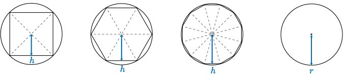
In \(300\) to \(200\) BC, Greek mathematicians used a method of exhaustion in hopes of finding the formula for the area of a circle. Greek mathematicians inscribed regular polygons within a circle.
You can see a circle, and inside the circle, a square has been inscribed.
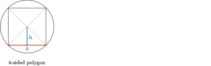
This square has been broken into four congruent triangles, each having height \(h\) and base \(b\). When we look at this diagram, we see that the square does an all right job of approximating the area of the circle. However, there is still quite a bit of white space around the square that is part of the area of the circle.
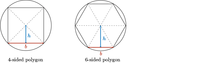
As we increase the sides of the polygon that is inscribed within the circle (for instance, take the \(4\)-sided square and instead inscribe a \(6\)-sided hexagon within this circle), we see that the hexagon does a better job of covering the area of the circle.
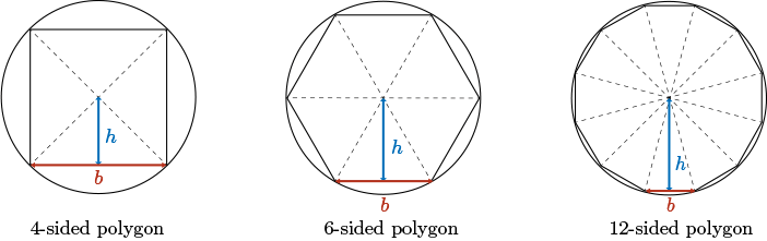
Continuing in this fashion, we could inscribe a polygon that has \(8\) sides, \(10\) sides, or \(12\) sides.
They divided each \(n\)-sided polygon into \(n\) congruent triangles.
As we progress from \(4\) to \(6\) to \(8\) to \(10\) to \(12\) sides, the polygon does a better job of approximating the area of the circle. With a \(12\)-sided polygon, we can barely see the white space that surrounds the polygon that lies within the circle. This is a very good approximation.
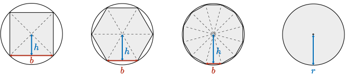
Now, the area of each of these polygons is easy to find if you break the polygon into, again, congruent triangles. So a \(6\)-sided polygon, we will break into \(6\) congruent triangles. The \(12\)-sided polygon, we break into \(12\) congruent triangles. We know how to find the area of a triangle. The area of a triangle is \(\dfrac{1}{2}bh\). So if we know the height and base of each triangular segment, we multiply that area by \(12\), we get the area of the entire polygon.
The area of each polygon can be found by multiplying the area of the triangles by \(n\).
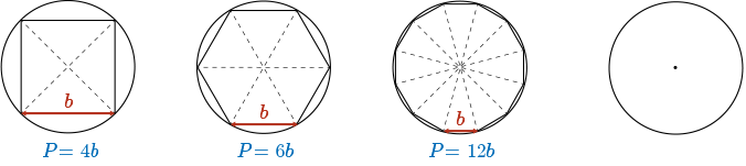
As the number of sides in the polygon inscribed within the circle increases, the perimeter, \(P\), of each polygon approaches (becomes closer in value to) the circumference of the circle \((2\pi r)\).
The perimeter, \(P\), of each polygon is calculated by multiplying the the number of sides in the polygon, \(n\), by the length of the base of each triangle, \(b\). This is approximately the same as \(2 \pi r\), a formula that the Greek mathematicians already knew for the circumference of the circle.
\(P=nb\) \( \approx 2\pi r\)
Also, as the number of sides in the polygon increases, the height, \(h\), of each triangle approaches the length of the radius of the circle.
As the number of sides in the polygon increases, we also see that the area of the polygon approaches the area of the circle.
When we look at the area of the circle covered by the \(4\)-sided polygon, the square, we see that it does, again, an all right job of approximating the area. As the number of sides in the polygon increases, we see that the polygon does a better and better job of approximating the area of the circle. Now look at the height again in this diagram. As we progress from a \(4\)-sided to a \(6\)-sided to a \(12\)-sided polygon, we see that the height of each triangular section within the polygon starts to resemble the length of the radius of the circle. And so since the height is approaching the value of the radius, we can say that they are approximately equal.
\[h \approx r\]
Lesson Part 2
Developing a Formula for the Area of a Circle
The Greek Method of Exhaustion (300-200 BC)
To calculate the area, \(A_n\), of the \(n\)-sided polygon, calculate the area, \(A_{triangle}\), of one triangular section and multiply this by the number of triangular sections in the polygon, which in this case is actually the same as the number of sides of the polygon \(n\).
Thus, the area of \(n\) sided polygon would be \(n\), the number of sides times the area of the triangle. Well, we know the formula for the area of the triangle.
\[A_n=nA_{triangle}\]
It's \(\dfrac{1}{2}bh\). So instead of writing area of triangle, we can substitute this formula in its place.
\[nA_{triangle}=n\left(\dfrac{1}{2}bh\right)\]
Rearranging this formula, since there is just multiplication between each of the variables and also the values in this expression, we can rearrange these values in variables however we please. So in this case, I'm going to lump together the number of sides \(n\) and the length of the base \(b\). I'm also going to lump together \(\dfrac{1}{2}\) and height.
\[n\left(\dfrac{1}{2}bh\right)=(nb)\left(\dfrac{1}{2}h\right)\]
Well, let's remember back. \(n\) times \(b\) was the form that we use to calculate the perimeter of the polygon. And remember, the perimeter of the polygon approached the circumference of the circle. And so we know that the perimeter, which equals \(n\) times \(b\), is approximately the same as \(2 \pi r\). So in its place, we're going to substitute \(2 \pi r\), the formula for the circumference of the circle. Also, we have seen that the height of each triangular section approaches the length of the radius of the circle. So we know that the height of each of the triangles sections becomes approximately the length of the radius of the circle. So where we originally had height, we're now going to substitute radius.
\[(nb)\left(\dfrac{1}{2}h\right) \approx (2\pi r)\left(\dfrac{1}{2}r\right) \text{ recall that } P=nb\approx 2\pi r \text{ and } h \approx r\]
If we simplify this expression, it simplifies to being the formula
\[A_n \approx \pi r^2\]
Putting it all together, we have
\[\begin{align*} A_n&=nA_{triangle} \\ &=n\left(\dfrac{1}{2}bh\right) \\ &=(nb)\left(\dfrac{1}{2}h\right) \\ &\approx (2\pi r)\left(\dfrac{1}{2}r\right) \text{ recall that } P=nb\approx 2\pi r \text{ and } h \approx r \\ &\approx \pi r^2 \end{align*}\]
The area, \(A_n\), of the polygon approaches the area of the circle, \(A_n \approx \pi r^2\), and this approximation becomes more accurate as \(n\) increases.
In other words, an n sided polygon has approximately the same area as the circle for very large values of \(n\). And as \(n\) becomes larger and larger in value, our approximation becomes more and more accurate.
This does not mean that these areas will ever be equal. Instead, the area of the polygon becomes closer in value to the area of the circle as the number of sides in the polygon increases.
Mathematicians use the term limit to identify approached values. A limit, again, does not necessarily mean that we equal a value. It means that we are approaching a value. So we could use the term limit in this case, since the area of a polygon approaches the area of the circle. They use the following expression to represent this:
\[\lim_{n\to\infty} A_n =A_{Circle}\]
where \(n\) is the number of sides in the polygon.
So we say the limit as \(n\) approaches infinity, meaning \(n\) is getting very, very large, of the area of a \(n\) sided polygon is equal to the area of a circle. Again, this does not say that the area of a polygon is equal to the area of the circle. It says that the area of the polygon is approaching the area of the circle. We know that, because we've included the term limit in front.
Lesson Part 3
Two Fundamental Problems of Calculus
Now that we understand the concept of the limit, we're going to use that idea to understand what is calculus. Calculus was born from two problems.
The Area Problem
The Tangent Problem
The Area Problem (Integral Calculus)
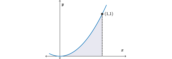
Mathematicians wanted to find the area under a curve. This is a very tough problem!
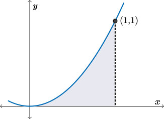
Much like we used polygons to approach the area of a circle in the introduction of this lesson, here, mathematicians used the sum of the areas of rectangles to help approximate the area under a curve.
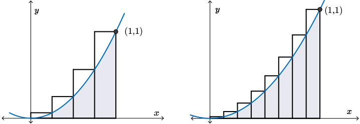
Image Description:
An image of the curve of the function \(f(x)=x^2\) from \(x=0\) to \(x=1\). Underneath the curve, there are four rectangles divided evenly between \(x=0\) and \(x=1\). Each rectangle starts at the \(x\)-axis and spans upwards until the top right corner of each rectangle touches the curve of \(f(x)=x^2\). A second diagram shows the same concept with eight rectangles instead of four.
When we look at the first diagram, we see that the rectangles do, again, an all right job of approximating the area under the curve. However, there is quite a bit of white space not covered by the area under the curve for each of the rectangles. As we decrease the width of each rectangle to get a better and better approximation of the area under the curve, we will need more rectangles in order to cover the entire area. As the number of rectangles increases or the width of each rectangle decreases, we see that we get a better and better approximation of the area under the curve.
As the width of the rectangle decreases (becomes very close to \(0\)), the sum of the areas of the rectangles, \(A_R\), would approach the area under the curve, \(A_C\).
If the width of each rectangle became very close to \(0\), not \(0\), but very, very close to \(0\) (meaning the rectangles would be very, very small, slender, sections), then the sum of the areas of the rectangles would approach the area under the curve. Again, we can use limits here to symbolize this idea.
This is written as
\[\lim_{w\to 0} A_R = A_C\]
which means that as the width of the rectangles becomes almost \(0\), the sum of the area of the rectangles approaches the area under the curve.
Lesson Part 4
Two Fundamental Problems of Calculus
The Tangent Problem (Differential Calculus)
The second problem involved in calculus is the tangent problem.
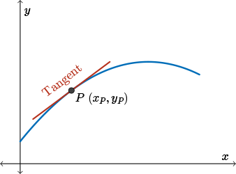
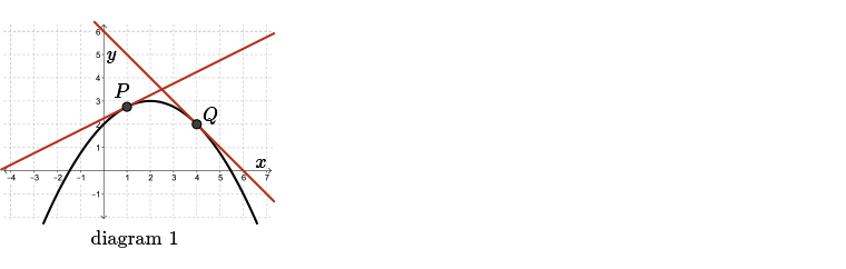
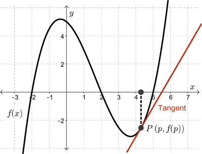
A tangent is a line which tells us how “steep” the curve is at the point of tangency.
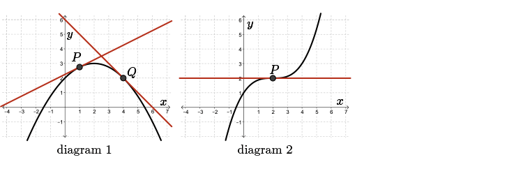
Look at the following diagram. There's a few ways a tangent line may be drawn to a curve. A tangent line may just “kiss” the curve, as at points \(P\) and \(Q\) in diagram \(1\).
A tangent line may cross through the curve, as at point \(P\) in diagram \(2\), where the curve changes from bending downwards to upwards or vice versa.
A curve may not always have a tangent line at each point, as at points \(P\) and \(Q\) in diagram 3, where the curve has a “sharp” point or “corner.”
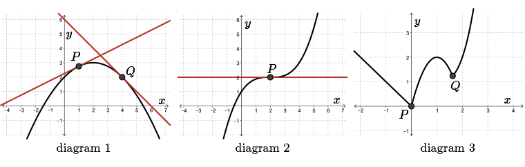
Since the function at this point drastically changes, actually instantaneously changes from curving one way to curving the other way, we can't draw a tangent at this point.
Before the invention of calculus, mathematicians wanted to find the equation of a tangent to a curve. You have formed the equation of a line before. You have formed the equation of a line before. To form the equation of the line, you need two pieces of information, the slope of the line and a point on the line.
Well, finding the equation of a tangent is very similar. To find the equation of the tangent, we must calculate the slope of the tangent and we'll also need the point of tangency, which is a challenging problem.
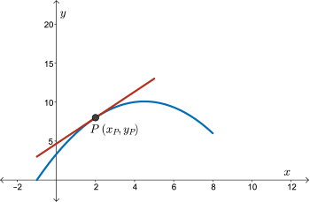
When we look at the original diagram of a tangent drawn to a curve, we see that the tangent goes through a point. But we do not have a second point on the tangent that will allow us to calculate its slope.
However, the slope of the tangent can be approximated by examining the slopes of the secants nearby this point.
Choose another point, \(Q\), on the curve that is nearby to \(P\).
Draw a secant between points \(P\) and \(Q\) and calculate the slope of this secant.
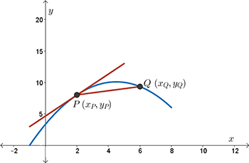
Now when we look at the secant drawn the curve, we see that, again, the secant does an all right job of approximating the slope of the tangent.
Well, how can we make the slope of the secant resemble the slope of the tangent better? Let's move point \(Q\) towards point \(P\).
As we move point \(Q\) towards point \(P\) and calculate the slope of each secant line, we notice that the slope of the secant approaches a certain value, which we take to be the slope of the tangent line.
We calculate the slope of the secant using the following formula. We subtract the \(y\)-coordinates of point \(P\) from the \(y\)-coordinate of point \(Q\), and then we divide that by the difference between the \(x\)-coordinate at point \(Q\) and the \(x\)-coordinate point \(P\).
\[\begin{align*}m_{PQ}&=\dfrac{y_Q - y_P}{x_Q-x_P} \\ &=\frac{f(x_Q)-f(x_P)}{x_Q-x_P}\end{align*}\]
We can use limits to symbolize the idea that the slope of the secant approaches the slope of the tangent.
\[\lim_{Q \to P} m_{PQ} = m_{tangent}\]
The limit of \(Q\) approaching \(P\) of \(m_{PQ}\), which is the slope of the secant \(PQ\), is equal to \(m_{tangent}\), the slope of the tangent.
Lesson Part 5
Rates of Change
Average Rate of Change
The tangent problem has many connections to real life applications. The strongest connection to real life is in average and instantaneous rates of change. Let's recall average rate of change.
The average rate of change of a function, \(f(x)\), over an interval, \(p \le x \le q\). For instance, if we started at point \(P\) and we ended at point \(Q\), we're looking at, how is the function changing within these two values? In this case, we use the slope of the secant to calculate average rate of change. The average rate of change is defined as
\[Rate_{average}=\frac{f(q)-f(p)}{q-p}\]
which is the slope of the secant \(PQ\).

Instantaneous Rate of Change
Instantaneous rate of change, though, is the rate of change at a particular instance on a function, so we're looking at only one point. In this case, we're looking at point \(P\).
The instantaneous rate of change is found by calculating the slope of the tangent. As we have seen, the slope of the secant approaches the slope of the tangent as point \(Q\) is dragged towards point \(P\), so the slope of the tangent at point \(P\) is the limit of the slope of the secant between points \(P~(p,f(p))\) and \(Q~(q,f(q))\).
We define this limit as the instantaneous rate of change of \(f(x)\) at \(x=p\).
Geometrically,
Application of Rates of Change
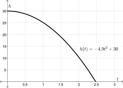
Let's use an example to demonstrate the difference between average and instantaneous rate of change. Suppose we are standing on a bridge, and we are holding a pebble in our hand. We drop the pebble, and the height of the pebble above the surface of the water is recorded at \(\dfrac{1}{2}\)-second increments until it hits the water.
The following graph shows the height, \(h(t)\), of a pebble above the surface of a river as a function of time, \(t\), after it is dropped from a bridge.
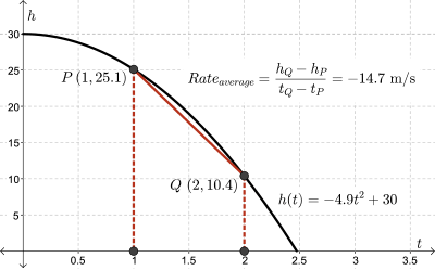
After the pebble is dropped, we can calculate the average speed of the falling pebble between \(1\) and \(2\) seconds by calculating the slope of the secant, \(PQ\), from time \(t = 1\) to \(t = 2\).
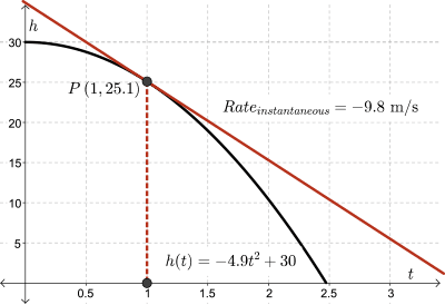
The instantaneous speed of the pebble exactly \(1\) second after it is dropped is found by calculating the slope of the tangent at point \(P\).
So how do we find the slope of the tangent?
The slope of the secant between points \(P\) and \(Q\) can be used to approximate the slope of the tangent. Here, point \(Q\) occurs when \(t = 2\).
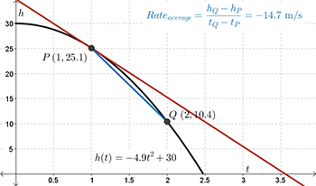
When we look at the diagram, we see that the slope of the secant, again, does an OK job of approximating the slope of the tangent.However, if we move point \(Q\) towards point \(P\), we are going to get a better and better approximation of the slope of the tangent.
Let's begin with point \(Q\) at \((2,10.4)\). The slope of the secant, \(PQ\), is \(-14.7\).
Moving point \(Q\) towards point \(P\) at intervals of \(0.1\), the slope of the secant becomes closer in steepness to the slope of the tangent.
The following table of values tracks the slope of the secant as point \(Q\) moves closer to point \(P\) at increments of \(0.1\).
| \[\Delta t\]\[(t_Q-t_P)\] |
\[\Delta h\]\[(h_Q-h_P)\] |
\(m_{PQ}=\dfrac{\Delta h}{\Delta t}\) |
| \(1\) |
\(-14.7\) |
\(-14.7\) |
| \(0.9\) |
\(-12.789\) |
\(-14.21\) |
| \(0.8\) |
\(-10.976\) |
\(-13.72\) |
| \(0.7\) |
\(-9.261\) |
\(-13.23\) |
| \(0.6\) |
\(-7.644\) |
\(-12.74\) |
| \(0.5\) |
\(-6.125\) |
\(-12.25\) |
| \(0.4\) |
\(-4.704\) |
\(-11.76\) |
| \(0.3\) |
\(-3.381\) |
\(-11.27\) |
| \(0.2\) |
\(-2.156\) |
\(-10.78\) |
| \(0.1\) |
\(-1.029\) |
\(-10.29\) |
As point \(Q\) is moved towards point \(P\), we see that the slope of the secant becomes more and more like the slope of the tangent. In the table of values, we've now gone from a slope of negative \(14.7\) to a slope of \(-10.29\) when point \(Q\) is only \(1/10\) of a unit of time from point \(P\).
To get a better approximation, let's zoom in on the graph and move point \(Q\) towards point \(P\) at intervals of \(0.01\) until point \(Q\) is just right of point \(P\).
| \[\Delta t\]\[(t_Q-t_P)\] |
\[\Delta h\]\[(h_Q-h_P)\] |
\(m_{PQ}=\dfrac{\Delta h}{\Delta t}\) |
| \(0.1\) |
\(-1.029\) |
\(-10.29\) |
| \(0.09\) |
\(-0.92169\) |
\(-10.241\) |
| \(0.08\) |
\(-0.81536\) |
\(-10.192\) |
| \(0.07\) |
\(-0.71001\) |
\(-10.143\) |
| \(0.06\) |
\(-0.60564\) |
\(-10.094\) |
| \(0.05\) |
\(-0.50225\) |
\(-10.045\) |
| \(0.04\) |
\(-0.39984\) |
\(-9.996\) |
| \(0.03\) |
\(-0.29841\) |
\(-9.947\) |
| \(0.02\) |
\(-0.19796\) |
\(-9.898\) |
| \(0.01\) |
\(-0.09849\) |
\(-9.849\) |
We now have values for the slope of the secant, \(PQ\), as point \(Q\) approaches point \(P\) on the right side.
So we started with the slope of the secant at \(-10.29\). When we are only \(\dfrac{1}{100}\) of a unit of time from a point \(P\), we see that the slope of the secant is \(-9.849\). We are approaching somewhere the value of \(-9.8\). But is it \(-9.8\)? Well, how can we convince ourselves of our approximation?
Let's now choose a point \(Q\) to the left of point \(P\) to observe how the slope of the secant approaches the slope of the tangent from the left side. Again, we know that as point \(Q\) approaches point \(P\), the slope of the secant approaches the slope of the tangent.
Let's begin at \(Q~(0.5, 28.79)\) and move point \(Q\) towards point \(P\) at intervals of \(0.1\).
| \[\Delta t\]\[(t_Q-t_P)\] |
\[\Delta h\]\[(h_Q-h_P)\] |
\(m_{PQ}=\dfrac{\Delta h}{\Delta t}\) |
| \(-0.5\) |
\(3.675\) |
\(-7.35\) |
| \(-0.4\) |
\(3.136\) |
\(-7.84\) |
| \(-0.3\) |
\(2.499\) |
\(-8.33\) |
| \(-0.2\) |
\(1.764\) |
\(-8.82\) |
| \(-0.1\) |
\(0.931\) |
\(-9.31\) |
The first slope of the secant is \(-7.35\). As we move point \(Q\) towards point \(P\), when we are only \(\dfrac{1}{10}\) of a unit of time from point \(P\), we see that the slope of the secant is \(-9.31\). This is a better approximation of the slope of the tangent.
Zooming in on the graph, let's move point \(Q\) towards point \(P\) at intervals of \(0.01\) until point \(Q\) is just left of point \(P\).
| \[\Delta t\]\[(t_Q-t_P)\] |
\[\Delta h\]\[(h_Q-h_P)\] |
\(m_{PQ}=\dfrac{\Delta h}{\Delta t}\) |
| \(-0.1\) |
\(0.931\) |
\(-9.31\) |
| \(-0.09\) |
\(0.84231\) |
\(-9.359\) |
| \(-0.08\) |
\(0.75264\) |
\(-9.408\) |
| \(-0.07\) |
\(0.66199\) |
\(-9.457\) |
| \(-0.06\) |
\(0.57036\) |
\(-9.506\) |
| \(-0.05\) |
\(0.47775\) |
\(-9.555\) |
| \(-0.04\) |
\(0.38416\) |
\(-9.604\) |
| \(-0.03\) |
\(0.28959\) |
\(-9.653\) |
| \(-0.02\) |
\(0.19404\) |
\(-9.702\) |
| \(-0.01\) |
\(0.09751\) |
\(-9.751\) |
OK, so let's recap. When point \(Q\) was \(\dfrac{1}{100}\) of a unit of time to the right of point \(P\), the slope of the secant was \(-9.849\). When point \(Q\) was \(\dfrac{1}{100}\) of a unit of time to the left of point \(P\), the slope of the secant was \(-9.751\).
We now have the progression of slopes for secant \(PQ\) as \(Q\) approaches \(P\) from the left and right sides.

By examining how the slopes of the secants change as we approach the middle of the table, our best approximation for the slope of the tangent is \(-9.8\) m/s, as this value lies between \(-9.849\) and \(-9.751\). However, this is still only an approximation of the slope of the tangent. We are not \(100\%\) sure that this is actually the slope of the tangent. We will see a method of calculating this slope exactly in lessons to come.
| \[\Delta t\]\[(t_Q-t_P)\] |
\[\Delta h\]\[(h_Q-h_P)\] |
\(m_{PQ}=\dfrac{\Delta h}{\Delta t}\) |
| \(0.07\) |
\(-0.71001\) |
\(-10.143\) |
| \(0.06\) |
\(-0.60564\) |
\(-10.094\) |
| \(0.05\) |
\(-0.50225\) |
\(-10.045\) |
| \(0.04\) |
\(-0.39984\) |
\(-9.996\) |
| \(0.03\) |
\(-0.29841\) |
\(-9.947\) |
| \(0.02\) |
\(-0.19796\) |
\(-9.898\) |
| \(\textcolor{NavyBlue}{0.01}\) |
\(-0.09849\) |
\(\textcolor{NavyBlue}{-9.849}\) |
| \(\textcolor{NavyBlue}{-0.01}\) |
\(0.09751\) |
\(\textcolor{NavyBlue}{-9.751}\) |
| \(-0.02\) |
\(0.19404\) |
\(-9.702\) |
| \(-0.03\) |
\(0.28959\) |
\(-9.653\) |
| \(-0.04\) |
\(0.38416\) |
\(-9.604\) |
| \(-0.05\) |
\(0.47775\) |
\(-9.555\) |
| \(-0.06\) |
\(0.57036\) |
\(-9.506\) |
| \(-0.07\) |
\(0.66199\) |
\(-9.457\) |
Lesson Part 6
Rates of Change
Calculating the Average Rate of Change for Any Function
So to recap, in calculating the average rate of change of any function, the average rate of change between two points is calculated by finding the slope of the secant between these two points on the curve.
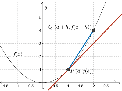
The point \(P~(a,f(a))\) is a point on the function \(y=f(x)\).
A second point, \(Q\), that is a horizontal displacement, \(h\), away from \(P\) has coordinates \(Q~(a+h, f(a+h))\).
We know how to calculate the slope of the secant. The slope of the secant is calculated by the difference of the \(y\)'s divided by the difference of the \(x\)'s. So in this case the slope of the secant is calculated by
\[m_{secant} = \dfrac{f(a+h)-f(a)}{(a+h)-a}\]
We can simplify the denominator in this expression to simply just be \(h\).
\[m_{secant} = \dfrac{f(a+h)-f(a)}{h}\]
Mathematicians refer to this formula as the difference quotient.
Calculating the Instantaneous Rate of Change for Any Function
The instantaneous rate of change at a point is calculated from the slope of the tangent at that point.
We have seen that the slope of the tangent can be approximated by considering the slopes of the secants from the point of tangency to nearby points.
In general, to find the slope of the tangent to the function \(y=f(x)\) at point \((a,f(a))\), choose a point that is a close horizontal displacement, \(h\), away.
This point has coordinates \((a+h, f(a+h))\).
The slope of the tangent is found by considering the slopes of secants as point \(Q\) moves closer to point \(P\).
In other words, the horizontal displacement between points \(Q\) and \(P\) approaches \(0\), meaning it is getting smaller and smaller and smaller. Thus we can use limits to show the formula for calculating the slope of the tangent.
The slope is defined by
\[m_{tangent} = \lim_{h \to 0} \frac{f(a+h)-f(a)}{(a+h)-a}\]
the limit of the difference quotient.
Again, we know that the denominator in this case can be simplified to just simply be \(h\). Here, we are performing the limit on the difference quotient.
Summary
In summary, we have the following theorem that can be used to find the slope of a tangent line.
Suppose \(f(x)\) is defined on an open interval containing \(c\), where \(\Delta y\) is defined to be \(f(c+h)-f(c)\), and \(\Delta x\) is defined to be \((c+h)-c=h\). Then if
\[\lim_{h \to 0} \frac{\Delta y}{\Delta x} = \lim_{h \to 0} \frac{f(c+h)-f(c)}{h}\]
exists, the line passing through \((c,f(c))\) with slope \(m\), equal to this limit, is the tangent to the graph of \(f(x)\) at the point \((c,f(c))\).
Lesson Part 7
Examples
Example 1
Let's try the following example together.
Approximate the slope of the tangent to the curve \(f(x)=\sqrt{x^2-25}\) at \(x=8\).
Solution
We have seen how to use the slopes and the secants between points to approximate the slope of the tangent. Let's do that here.
Calculate the slopes of secants from point \(P\) where \(x=8\) to points \(Q\) which are nearby, by adding and subtracting \(0.1\), \(0.01\), and \(0.001\) from \(x=8\), to get values of \(x\) to the right and left of point \(P\).
Again, we will use a table to organize our values. Now the tangent is drawn when \(x = 8\). So this is point \(P\). This is the point that remains fixed throughout all of our calculations. So the slope of secant between a point \(Q\) and point \(P\), will be calculated by \(m=\dfrac{f(x_Q)-f(8)}{x_Q-8}\).
The completed table of values should be as follows:
| \(x_Q\) |
\(f(x_Q)=\sqrt{x_Q^2-25}\) |
Slope of Secant \(PQ\) |
| \(7.9\) |
\(6.11637147\) |
\(1.28626525\) |
| \(7.99\) |
\(6.2321826\) |
\(1.281539517\) |
| \(7.999\) |
\(6.24371692\) |
\(1.281076564\) |
| \(8.001\) |
\(6.24627897\) |
\(1.280973918\) |
| \(8.01\) |
\(6.25780313\) |
\(1.28051305\) |
| \(8.1\) |
\(6.37259759\) |
\(1.275995881\) |
By examining the table of values and slopes of secant, we see that as point \(Q\) approaches point \(P\) from the left and right side, the slope of the secant appears to approach the value \(1.281\) approximately. So this is the value that we will use for the slope of the tangent.
Example 2
Calculate the slope of the tangent to the curve \(f(x)=x^2-6\) at \(x=2\).
Solution
We want to calculate the slope of the tangent at \(x = 2\). So our point of tangency is \((2,f(2))\). Let's label this as point \(P\). Now let's choose another point, say point \(Q\), that has a displacement away from point \(P\). It's coordinates would be \((2 + h,f(2+h))\).
If \(P\) is the point \((2,f(2))\) and \(Q\) is \((2+h, f(2+h))\), then the slope of the secant is
\[\begin{align*}m_{secant}&=\dfrac{\Delta f(x)}{\Delta x}\\ &=\dfrac{f(x_Q)-f(x_P)}{x_Q-x_P}\\ &=\dfrac{((2+h)^2-6)-((2)^2-6)}{(2+h)-2}\\ &=\dfrac{((h^2+4h+4)-6)-(4-6)}{h}\\ &=\dfrac{h^2+4h}{h}\\ &=h+4\end{align*}\]
We subtracted the \(y\)-coordinate of point \(P\) from point \(Q\) and we subtracted the \(x\)-coordinates. We then expanded and simplified the numerator. Notice the common factor of \(h\) in both terms in the numerator. We removed this common factor and canceled it with the denominator. Since we know \(h\) is not \(0\), it is approaching \(0\), we have the expression \(h + 4\).
As point \(Q\) approaches \(P\), the value \(h\) that was added to \(x\) becomes very small (i.e., approaches \(0\)).
Thus, the slope of the tangent to any point on the function is found by calculating the limit as \(h\) approaches \(0\) for the slope of the secant. Well, we know that the slope of the secant has been reduced to the expression \(h + 4\), so if \(h\) was getting very, very close to \(0\), imagine \(0.1\), \(0.01\), \(0.00001\). If we were to add this value to \(4\), essentially we have just \(4\). So we can really think of this as directly substituting \(0\) in for \(h\), even though \(h\) is not equal to \(0\), but it's really really close. If we add that amount to \(4\), we have the answer \(4\).
Putting it all together, we have
\[\begin{align*}m_{tangent}&=\displaystyle\lim_{h \to 0} m_{secant}\\ &=\displaystyle\lim_{h \to 0} (h+4)\\ &=(0)+4\\ &=4\end{align*}\]
Thus, the slope the tangent is 4.
Quiz
See the quiz in the side navigation.