Alternative Format

Try This

Different Approaches to Probabilities

The following spinner is spun. What is the probability that the spinner lands on yellow?

We can approach this problem in different ways through experimentation or using logic or theory.

Experimentally, we can perform a number of spins, or in other words, run a number of trials and record the outcome of each trial.

Experimentally

	Red	Yellow	Blue
Frequency	\(19\)	\(44\)	\(37\)

We want to determine for what fraction of the total trials the spinner lands on yellow. To do so, we divide the number of favorable trials by the total number of trials. According to this data, we estimate that the probability of landing on yellow is

\(\dfrac{\text{Favourable Trials}}{\text{Total Trials}} \class{timed in5}{= \dfrac{44}{100}} \class{timed in6}{=44\%}\)

Theoretically, we can measure the relative sizes of the different sections of the spinner and determine from this how likely it is the spinner lands on yellow. 

The spinner has \(8\) equally sized sections.

Theoretically

Since exactly \(3\) of these sections are yellow, we conclude that the probability that the spinner will land on yellow is \(\dfrac{3}{8}\) or \(37.5\%\).

Lesson Goals

• Compare the theoretical probability of an event to probability estimates found through experimentation.
• Explore how the number of trials performed in an experiment might impact the probability estimates, or experimental probabilities..

Try This!

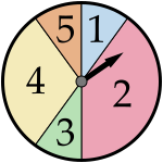
I have the following two spinners.

I will choose one of these spinners randomly and spin this spinner \(10\) times in a row, recording the outcome of each spin. Your task is to guess which spinner I used.

1. In one round of the game, the outcomes of my \(10\) spins are as follows:\[4, ~3, ~2, ~4, ~4, ~1, ~4, ~2, ~3, ~2\] Can you guess which spinner I used? Explain.
2. Is there a way to change this game to make you more confident in your guess?

Think about this problem, then move on to the next part of the lesson.

Differences Between Experiment and Theory

Try This Problem Revisited

Solution — Part 1

Let's reorder and group the outcomes. This will allow us to see the distribution of results a bit clearer. Now, how do these results compare to what you might have expected to see for each spinner?

\[1,~2,2,2,~3,3,~4,4,4,4\]

If we spun each spinner \(10\) times, we might expect the results for spinner one to be something close to the following list of outcomes in some order.

Spinner 1  

\[\class{timed add4-hl2 remove5-hl2}{1,1},~\class{timed add5-hl2 remove6-hl2}{2,2,2},~\class{timed add4-hl2 remove5-hl2}{3,3},~\class{timed add5-hl2 remove6-hl2}{4,4,4}\]

Since the sections for \(1\) and \(3\) appear to be equal in size, we might expect the spinner to land on each of these around the same number of times. Since the sections for \(2\) and \(4\) appear to be equal in size and a bit larger than the sections for \(1\) and \(3\), we might expect the spinner to land on each of these around the same number of times and a bit more often than one in three.

Using similar reasoning, we might expect the results for spinner two to be close to this list of outcomes in some order. Take a look and see if you agree based on the sections on Spinner 2.

• Spinner 2  \[1,~ 2,2,2,2,~3,~4,4,4,~ 5\]

It appears that the actual results look closer to what you might expect for Spinner 1. In particular, I didn't land on a section marked \(5\), which might suggest that I used Spinner 1. 

Are you comfortable declaring that I used Spinner 1? Would you be surprised if I told you I actually used Spinner 2?

Solution — Part 2

Is there a way to change this game to make you more confident in your guess? 

Recall the spinners:

I want to start by asking a slightly different question. If I was instead instructed to spin the chosen spinner \(100\) times, would you be more confident in your guess based on my results?

Well, I used the same spinner again, and here are my results for my \(100\) spins. Here, the first column of the table indicates the particular section label of the spinner. Let's compare these to what we would expect the results to be if we use the theoretical probabilities of the spinners.

	Actual Results
1	\(12\)
2	\(46\)
3	\(11\)
4	\(25\)
5	\(6\)

Based on the relative sizes of the sections on the spinner, we might expect the following distribution of results for spinner one and for spinner two.

	Expected Results (Spinner 1)	Expected Results (Spinner 2)
1	\(20\)	\(10\)
2	\(30\)	\(40\)
3	\(20\)	\(10\)
4	\(30\)	\(30\)
5	\(0\)	\(10\)

Comparing the three columns of data, it appears that the actual results look closer to what we might expect for Spinner 2.

In fact, you don't have to guess anymore. Since I spun a \(5\), you can be sure that I used Spinner 2.

This guessing game is all about trying to match what we see through experimentation to what we might expect to happen in theory. By studying theoretical probabilities, we can get an idea of what we think we should see if we spun spinner one a bunch of times or spinner two a bunch of times.

Now, random experiments rarely behave exactly how we might predict, but we will see that the number of trials in our experiments can have an effect on our probability estimates.

Example 1

Solution

The best way to do these activities is to actually get a coin out and try this yourself!

In fact, you may have already performed these activities in another lesson. If you do have your data ready to go, then that is great. 

If not, then you can use the exploration that follows which uses a "virtual" fair coin to perform the activities. We will pool data, so you will get \(1000\) trials to examine in part C.

Explore This 1

Description

Explore how the experimental probability of tossing heads changes depending on how many times the experiment is run.

Sample Experiment

Sample Summary of the Results

\(10\) Tosses	60%	50%	40%	30%	40%	60%	60%
\(50\) Tosses	50%	48%	38%	48%	60%	46%	44%
\(1000\) Tosses	51.2%	50.6%	52.4%	48.9%	51.7%	47.5%	52%

What do you notice when you look at how the experimental probabilities in each row compare to the theoretical probability of tossing heads?

Online Version

https://ggbm.at/hqa9aqae

Example 1 Continued

Solution

From the specific data given:

• None of the experimental probabilities match the theoretical probability of tossing heads, which is \(50\%\).
• The experimental probabilities got closer to \(50\%\) as the number of tosses increased.

What you might have observed while experimenting:

• Increasing the number of tosses does not guarantee an experimental probability that is closer to the theoretical probability. You may have seen probabilities equal to, or at least quite close to, \(50\%\) for only \(10\) tosses.
• Experimental probabilities between \(48\%\) and \(52\%\) were much more common for \(1000\) tosses than for \(10\) tosses.

Check Your Understanding 1

Question — Part A

A fair coin is tossed. What is the probability of tossing heads? 

Answer — Part A

The theoretical probability is \(50\%\).

Question — Part B

The fair coin is tossed \(50\) times and \(1000\) times. The tables summarize the results. 

In each case, what is the experimental probability of tossing heads?

Answer — Part B

Experiment 1:  \(\dfrac{20}{50} = 40\%\)

Experiment 2: \(\dfrac{495}{1000} = 49.5\%\)

Feedback — Part B

The probability after \(50\) trials is \(\dfrac{20}{50}\) or \(0.4\). 

The probability after \(1000\) trials is \(\dfrac{495}{1000}\) or \(0.495\).

Question — Part C

Choose the experiment for which the experimental probability is closer to the theoretical probability.

Answer — Part C

Experiment 2

Online Version

https://ggbm.at/ahuwqnuf

Increasing the Number of Trials

Tossing All Heads

You toss a fair coin many times in a row. What is the probability of tossing all heads?

This depends on the number of coin tosses. What if you

• tossed a coin twice and got \(2\) heads? I wouldn't be surprised.
• tossed a coin \(5\) times and got \(5\) heads? I would be quite surprised.
• tossed a coin \(100\) times and got \(100\) heads? I would start to wonder if your coin is really fair, or even if both sides of your coin might be marked with heads.

We start to feel like, as we toss a fair coin more and more times, the tosses should even out. This intuition is reflected in the theoretical probability calculations. There is a \(25\%\) chance that you will toss \(2\) heads in a row. There is only around a \(3\%\) chance that you will toss \(5\) heads in a row. So this is a pretty unlikely event, but not unheard of.

So what are your chances of tossing \(100\) heads in a row theoretically? Well, this probability is so close to \(0\) that it is tough to write down using decimal notation. It would be a decimal followed by \(30\) zeros! So we'll say it's very, very close to \(0\). It turns out that not only is it almost impossible to toss \(100\) heads in a row, but we can say more about the likely results after \(100\) tosses.

Number of Tosses	Probability of Tossing All Heads
\(1\)	\(50\%\)
\(2\)	\(25\%\)
\(3\)	\(12.5\%\)
\(4\)	\(6.25\%\)
\(5\)	\(3.125\%\)
\(100\)	Close to \( 0 \%\)

The Law of Large Numbers

If you toss a fair coin \(100\) times, then it would be almost impossible to toss \(100\) heads. Can we say more than that?
Certainly, heads might dominate for the first few tosses. But if you perform enough trials, then will the number of heads and tails be close to equal?

To answer this question, we turn to a very important phenomenon in probability theory that is often referred to as the law of large numbers.

If you think about it, experimental probabilities are estimates of the theoretical probability of an event.

These estimates will get closer to the theoretical probability as we increase the number of trials.

This law states that these estimates will get closer and closer to the theoretical probability as we increase the number of trials in our experiments. Going back to our coin toss example, when estimating the probability of tossing heads through experimentation:

• You may often get values larger than \(60\%\) or smaller than \(40\%\) over \(5\) or \(10\) tosses.
• It would be very uncommon to get values larger than \(60\%\) or smaller than \(40\%\) over \(50\) or \(100\) tosses.

Explore This 2

Description

Explore what happens to the frequencies of the rolls of a standard die and tosses of a coin as we allow for more trials.

Coin

\(1\) Trial

\(10\) Trials

\(100\) Trials

\(500\) Trials

Die

\(1\) Trial

\(10\) Trials

\(100\) Trials

\(500\) Trials

Created with GeoGebra. Author: University of Waterloo. CC BY-NC-SA 4.0. https://ggbm.at/z99mbbaa

Online Version

https://ggbm.at/z99mbbaa

Example 2

Solution

Now I want you to think about these questions carefully and come up with your answers and explanations to support them.

It might be tempting to think that the law of large numbers plays a role here. We have discussed how tossing all heads would be very unlikely if we performed six tosses. 

1. The two outcomes are equally likely to occur.
   All \(64\) possible outcomes of tossing a fair coin \(6\) times are equally likely to occur. These two outcomes are two of these possible outcomes. Even though getting all heads is less likely than getting some kind of mix of heads and tails, these two particular outcomes are equally likely to occur.
2. The probability of tossing tails on the sixth toss  is \(50\%\) as usual.
   Since each coin toss is independent of each other toss, the fact that the first five tosses came up heads has no effect on the probability of tossing tails on the sixth toss.

It is important to note the law of large numbers does not play a role when answering these particular questions. If we toss \(5\) heads in a row, then the coin doesn't magically know that we're really expecting tails next and change its weighting to be biased towards tails. But if we toss the coin enough times, then we will see the experimental probabilities get closer to \(50\%\).

This means, that if given enough trials, we seem to recover from experiments that start off dominated by heads. This happens even though we always have a fair chance of tossing heads or tails on every toss. This might feel like a bit of a brainteaser.

Check Your Understanding 2

Question

Which of the following statements are supported by the law of large numbers for a spinner with \(3\) equal sections coloured red, yellow, and blue? Select all that apply.

1. If you spin the spinner \(5\) times, then you will spin at least one colour other than yellow.
2. If you spin the spinner \(822\) times, then it is likely you will land on yellow close to \(274\) times.
3. If you spin the spinner \(858\) times, then the experimental probability of landing on yellow will likely be close to \(33.3\%\).
4. If you spin the spinner \(726\) times, then you will land on yellow exactly \(242\) times.

Answer

2. If you spin the spinner \(822\) times, then it is likely you will land on yellow close to \(274\) times.
3. If you spin the spinner \(858\) times, then the experimental probability of landing on yellow will likely be close to \(33.3\%\).

Feedback

The law of large numbers states that as the number of trails increases, the experimental probability of an event tends to get closer to the theoretical probability of the event.

The law of large numbers does not guarantee any results. It gives information about the results we can generally expect if we run a large number of trails.

Is Implied by the Law of Large Numbers

• If you spin the spinner \(822\) times, then it is likely you will land on yellow close to \(274\) times.
• If you spin the spinner \(858\) times, then the experimental probability of landing on yellow will likely be close to \(33.3\%\).

Is Not Implied by the Law of Large Numbers

• If you spin the spinner \(5\) times, then you will spin at least one colour other than yellow.
• If you spin the spinner \(726\) times, then you will land on yellow exactly \(242\) times.

Further Examples

Example 3

Solution

The theoretical probability of landing on red is \(\dfrac{1}{6}\) or \(16.\overline{6}\%\).

So if we spun the spinner many, many times, then we would expectthe number of times the spinner lands on red to be around \(\dfrac{1}{6}\) ofthe total number of spins.

1. \(6\) Spins

   We might expect \(1\) out of \(6\) spins to land on red.

2. \(600\) Spins

   We might expect \(100\) out of \(600\) spins to land on red.

Example 3 Continued

Solution

3. \(2\) more red than expected

   • If we land on red ‌\(2\) more times than we expect out of \(6\), then this would mean landing on red \(3\) out of \(6\) times.
     Suppose \(3\) out of \(6\) spins landed on red.
     This gives an experimental probability of \(50\%\).
   • If we land on red \(2\) more times than expected out of \(600\), then this would mean landing on red \(102\) out of \(600\) times.
     Suppose \(102\) out of \(600\) spins landed on red.
     This gives an experimental probability of \(17\%\).

What do we learn from these calculations?

Two more occurrences of red out of \(6\) produce an experimental probability that is nowhere near the theoretical probability of around \(16.7\%\). On the other hand, two more occurrences of red out of \(600\) produced an experimental probability that was essentially the same as the theoretical probability.

Getting a few more (or a few less) occurrences than expected has a large effect on the probability estimates in an experiment with few trials, but has almost no effect on the probability estimates in an experiment with many trials. As the number of trials continues to increase, this effect will become smaller and smaller and smaller.

Check Your Understanding 3

Question — Part 1

If a standard die is rolled once, the probability of rolling an even number is \(\dfrac{3}{6} = 50\%\).

1. If you were to roll the die \(6\) times, how many times would you expect to roll an even number?
2. If you were to roll the die \(66\) times, how many times would you expect to roll an even number?

Answer — Part 1

1. \(3\) times
2. \(33\) times

Feedback — Part 1

1. If you rolled the die \(6\) times, you might expect to roll an even number \(\dfrac{3}{6} = 3\) times.
2. If you rolled the die \(66\) times, you might expect to roll an even number \(\dfrac{3}{6} = 33\) times.

Question — Part 2

If you ran each of these experiments, and there were \(3\) more even numbers than expected, calculate the experimental probability of rolling an even number in each experiment.

Answer — Part 2

1. Experimental probability after \(6\) trials: \(\dfrac{6}{6} = 100\%\)
2. Experimental probability after \(66\) trials: \(\dfrac{36}{66} = \dfrac{6}{11} \approx 55\%\)

Feedback — Part 2

Since there were \(3\) more even numbers than expected, there were \(6\) favourable outcomes in the first experiment and \(36\) favourable outcomes in the second experiment.

Therefore, the experimental probability after \(6\) trials is \(\dfrac{6}{6}\) or \(1\) and after \(66\) trials is \(\dfrac{36}{66}\) or \(\dfrac{6}{11}\).

Notice that getting \(3\) more even numbers than expected affects the experimental probability more significantly when there are \(6\) trials.

Online Version

https://ggbm.at/xabg7pem

Example 4

Solution

Outcomes

• \(4\) outcomes for the die
• \(3\) outcomes for the spinner

There are \(12\) possible outcomes of this experiment. You can confirm this with a table, a list, or a tree diagram.

The roll and the spin are independent, and each of the \(12\) outcomes is equally likely to occur.  Only \(1\) outcome is favourable, so the probability is \(\dfrac{1}{12}\). If we spun the spinner \(12\) times, then we might expect to see this outcome once. Although, this is certainly not guaranteed.

The roll and the spin are independent and each outcome is equally likely to occur.

Unfortunately, there is no number of trials that will guarantee observing this particular outcome.

Appealing to the law of large numbers, we might choose to perform at least \(100\) trials, as it is extremely unlikely that we will not have seen this outcome at least once by then.

If you have the patience, you could invest in, say, \(1000\) trials. Then, seeing this outcome is essentially certain.

Take It With You

Jenny and Oscar would like to determine the sizes of all of the sections on their spinners without actually measuring the angles forming the sections.

1. Explain how to run an experiment to estimate the sizes of the sections on each spinner. 
2. Jenny and Oscar both know that a larger number of trials will mean that experimental probabilities will tend to be closer to theoretical probabilities. 
   Jenny claims that she does not need to do as many trials as Oscar to get reliable results for Question 1.
   Do you agree with Jenny? Explain.