Alternative Format — Lesson 6: Applications of Sinusoidal Functions

Let's Start Thinking 

Sinusoidal Functions in the Real World

In the last lesson of this unit, we will examine real-world situations that can be modelled by sinusoidal functions. There will be a little bit of astronomy and weather, some mechanics and ecology, as well as some fun experiences.

Sun rising over the crest of the earth, seen from space 

Canadian lynx on the prowl

A Ferris wheel

These scenarios are merely a taste of some applications were sinusoidal functions can be used to predict behavior and gain insight into the properties of these situations.


Lesson Goals

  • Relate the properties of sinusoidal functions to the characteristics of real-world situations.
  • Determine a sinusoidal function to model data that demonstrates periodic behaviour.

Try This

The average daily temperatures for each month in Winnipeg, Manitoba, Canada are in the table below.

Month Jan Feb March April May June July Aug Sep Oct Nov Dec
High (\(^\circ\)C) \(-10\) \(-8\) \(0\) \(11\) \(17\) \(23\) \(26\) \(25\) \(20\) \(11\) \(2\) \(-8\)
Low (\(^\circ\)C) \(-18\) \(-17\) \(-9\) \(0\) \(7\) \(13\) \(16\) \(15\) \(10\) \(3\) \(-6\) \(-15\)
  1. Write sinusoidal functions to model the average daily high temperatures and the average daily low temperatures.
  2. Compare the properties of the functions. Describe why some properties are similar and others are different.

Applications


In this section, we examine natural phenomena and engineered products that can be modelled by sinusoidal functions.

Ecology: Predator-Prey Interaction

In the wild, the population of two species may be related.

Predators

A lynx.

A predator hunting for food influences the population of its prey.

  • The more predators there are, the more likely the prey will be eaten.
  • The fewer predators, the more likely the prey are to survive and reproduce.

Prey

A snowshoe hare in the grass

The prey also affects the population of the predator.

  • The more prey, the more food available so the healthier the predators may become to catch prey and to reproduce.
  • The fewer prey, the less likely predators are to find food and survive or reproduce.

Historical Fact

The earliest evidence of a predator-prey interaction cycle was found in the records of the Hudson's Bay Company, in what is now part of northern Canada. The graph shows the number of pelts of snowshoe hare (Lepus americanus) and Canadian lynx (Lynx canadensis) the company bought from trappers between 1845 and 1935.

Graphs of pelt sales of Canadian Lynx and Showshoe Hare 1845-1935. Both graphs rise and fall in an approximately sinusoidal manner. The peaks of the lynx graph appears to be phase-shifted to the right, with respect to the hare graph.

Note: This data does not represent the actual populations of the two species during this time. It may be an indicator of the populations, since it is likely that trappers were able to sell more pelts to the company when the animal populations were higher and sold fewer pelts when the populations were lower.

Note: The degree symbol is not used in many of the sinusoidal functions in this lesson as the context of the application may require different units.

Example 1

The island of Nohumans is inhabited only by hare and lynx. Scientists began studying the populations of the two species in the year 2000 and have made the following population models:

\[\text{Hare: }H\left(t\right)=20\sin\left(45t\right)+60\]\[\text{Lynx: }L\left(t\right)=4.5\sin\left(45\left(t-2\right)\right)+8.5 \]

where the population of each species, \(H(t)\) and \(L(t)\), is measured in thousands and time (\(t\)) is measured in years since the year 2000.

  1. What was the maximum hare population? In which years was the hare population at a maximum?
  2. In what years was the lynx population at a maximum?
  3. Why are the years found in parts a) and b) the same or different?

Solution — Part A

For a sinusoidal function of the form \(y=a\sin\left(b\left(x-h\right)\right)+k\), the maximum value of the function is \(k+\lvert a\rvert\).

From the model, \(H\left(t\right)=20\sin\left(45t\right)+60\), the maximum population was \(20~000+60~000=80~000\) hare.

To determine in which years the hare population was at a maximum, we need to solve for \(t\) in the equation:

\[\begin{align*} 20\sin\left(45t\right)+60&=80\\ 20\sin\left(45t\right)&=20\\ \sin\left(45t\right)&=1 \end{align*}\]

The base sine function reaches its maximum value of \(1\) when the input is \(90\) and repeats regularly since for all \(n\in\mathbb{Z}\), \(\sin\left(\left(90+360n\right)\right)=1\). Equating the inputs of the two equations, we get

\[\begin{align*} 45t&=90+360n\\ t&=2+8n \end{align*}\]

Therefore, the hare population was at a maximum in the years 2002, 2010, 2018, and every \(8\) years afterwards.

Solution — Part B

Method 1: Compare Period and Phase Shift

Comparing the hare model \(H\left(t\right)=20\sin\left(45t\right)+60\) and the lynx model \(L\left(t\right)=4.5\sin\left(45\left(t-2\right)\right)+8.5\), the two sine functions have the same \(b\) value but different \(h\) values. The period of both models is \(\dfrac{360}{45}=8\) years but the lynx model has a phase shift of \(2\) years to the right. This means that the lynx will reach their maximum population \(2\) years after the hare reach their maximum population, or in the years 2004, 2012, 2020, and every \(8\) years afterwards.

Method 2: Solve Equation

The maximum lynx population of \(4500+8500=13~000\) occurs when 

\[\begin{align*} 4.5\sin\left(45\left(t-2\right)\right)+8.5&=13\\ 4.5\sin\left(45\left(t-2\right)\right)&=4.5\\ \sin\left(45\left(t-2\right)\right)&=1 \\ \text{Since }\sin\left(90+360n\right)&=1 \text{ for }n\in\mathbb{Z}\\ 45\left(t-2\right)&=90+360n\\ t-2&=2+8n \\ t&=4+8n \end{align*}\]

Therefore, the maximum lynx population occurs in the years 2004, 2012, 2020, and every \(8\) years afterwards.

Solution — Part C

Predator-prey interaction says that the more prey, the healthier the predators may become to catch prey and to reproduce. This implies that there is a delay between when the hare reach their maximum population and food is abundant for the lynx and when the lynx population reproduces to reach its maximum. From the models, this delay is \(2\) years.

Math In Action

Sinusoidal predator-prey models are simple examples of Lotka-Volterra equations that are used to describe the interactions of two species. Researchers apply these models to the following fields of study:

  • Agriculture: weeds and insects (prey), herbicides and pesticides (predator)
  • Medicine: disease (prey), drug (predator)

There is a body of thought that applying pesticides or giving patients medicine periodically rather than constantly may reduce the risk of treatment side effects, may reduce the risk of developing chemical resistance, and may reduce the cost of treatments. More research is needed to test these hypotheses.

Ocean Cycles

Did You Know?

The point on the Earth closest to the Moon is called the sublunar point.

The point on the Earth farthest from the Moon is called the antipodal point.

While our Earth is close to spherical, the world's oceans bulge in two areas, one around the sublunar point and the other around the antipodal point. These points are constantly moving as the Earth makes its daily rotation on its axis, and as the Moon rotates around the Earth every 28 days. It turns out that a particular point on Earth will be a sublunar point every 24 hours and 50 minutes.

The moon revolves around the Earth as the Earth rotates to the East. The sublunar point is seen to be the point on Earth closest to the moon. The antipodal point is seen to be the point on Earth farthest from the moon. Both of these points exhibit ocean swelling due to high tides.

Example 2

The depth of the water in a harbour, \(D\left(t\right)\), in metres, can be estimated by the function \(D\left(t\right)=4.3\cos\left(29t\right)+7\), where \(t\) is the number of hours after high tide.

  1. Identify the values of \(a\), \(b\), and \(k\) and interpret their meaning in this situation.
  2. If high tide occurred at 5:00 AM. Determine the depth of the water at
    1. 9:00 AM, and
    2. 2:45 PM.

Solution — Part A

From the equation \(D\left(t\right)=4.3\cos\left(29t\right)+7\), we know \(a=4.3\), \(b=29\), and \(k=7\).

  • The value \(k=7\) means that the average water depth in the harbour is \(7\) m.
  • The amplitude is \(4.3\) so the height of the water could be up to \(4.3\) m away from the average or between \(7-4.3=2.7\) m and \(7+4.3=11.3\) m.
  • The period is \(\dfrac{360}{29}\approx12.41\) hours. This means that high tide occurs approximately every \(12\) hours and \(25\) minutes.

Solution — Part B

  1. Since high tide occurred at 5:00 AM, 9:00 AM is \(4\) hours later.\[\begin{align*} D\left(4\right)&=4.3\cos\left(29\left(4\right)\right)+7\\ &=5.115\ldots \end{align*}\]

    At 9:00 AM, the water was approximately \(5.1\) m deep.

  2. From 5:00 AM to 2:00 PM is \(9\) hours, so 2:45 PM is \(9 + 0.75 = 9.75\) hours after high tide.\[\begin{align*} D\left(9.75\right)&=4.3\cos\left(29\left(9.75\right)\right)+7\\ &=7.948\ldots \end{align*}\]

    At 2:45 PM, the water was approximately \(7.9\) m deep.


Check Your Understanding 1

Question

The position of a rider on a Ferris wheel is modelled by the sinusoidal function. 

\[h\left(t\right)=-14\cos\left(90 t\right)+16\]

where \(h\left(t\right)\) is the rider's height in metres above the ground and \(t\) is the time in minutes from when the ride begins.

  1. If the ride is \(12\) minutes long, how many revolutions does the rider make on the wheel? 
  2. What was the rider's height after \(9\) minutes? Round your answer to the nearest tenth of a metre.

Answer

  1. Number of revolutions \(=3\)
  2. \(16\)

Feedback

  1. The period of the function is \(\dfrac{360}{90}=4\) minutes for one revolution, so the number of revolutions of the ride is \(12 \div 4=3\).
  2. To find the rider's height after \(9\) minutes, substitute and evaluate

    \(\begin{align*}h(9)=-14 \cos (90(9))+16=16 \end{align*}\)

    The rider's height was \(16.0\) m.


Electric Facts

Did You Know?

Alternating current (AC for short) is an electric current that regularly reverses the direction of its charge many times each second.

  • The described voltage of a charge is the maximum voltage of the charge multiplied by \(\dfrac1{\sqrt2}\). The described voltage is technically called the root-mean-squared (rms) voltage.
  • In one cycle, the charge changes its direction twice. The frequency, in Hertz (Hz), is the number of cycles per second.

The electric current that powers many homes in North America is described to have a voltage of \(120\) V and a frequency of \(60\) Hz.

A North American electrical outlet

In many other parts of the world, the current is described to have a voltage of \(220\) V and a frequency of \(50\) Hz.

A European electrical outlet

Example 3

The voltage, \(N\left(t\right)\) in volts, of a North American alternating current can be modelled by the function \(N\left(t\right)=170\sin\left(21\,600t\right)\), where \(t\) is time measured in seconds.

  1. Show that this model function has a described voltage of \(120\) V and a frequency of \(60\) Hz.
  2. Write a function to model the voltage, \(W\left(t\right)\), of an alternating current with a described voltage of \(220\) V and a frequency of \(50\) Hz .

Solution — Part A

Voltage

The maximum voltage of the model is the amplitude, \(170\) V.

According to the Did You Know, 

\[\begin{align*} \text{Described Voltage }&=\dfrac1{\sqrt{2}}\times\text{Maximum Voltage}\\ &=\dfrac1{\sqrt2}\left(170\right)\\ &=120.2081\ldots \end{align*}\]

The described voltage for the model function is approximately \(120\) V.

Frequency

The model function has \(b=21~600\), so the period of the model is \(\dfrac{360}{\lvert b\rvert}=\dfrac{360}{21\,600}=\dfrac1{60}\) seconds. In one second, the model would have \(60\) cycles or a frequency of \(60\) Hz.

Solution — Part B

Voltage

For a described voltage of \(220\) V,

\[\begin{align*} \text{Described Voltage }&=\dfrac1{\sqrt{2}}\times\text{Maximum Voltage}\\ 220&=\dfrac1{\sqrt2}\left(\text{Maximum Voltage}\right)\\ \text{Maximum Voltage}&=220\sqrt2\\ &=311.1269\ldots \end{align*}\]

The maximum voltage is approximately \(311\) V, which will be the amplitude of the model function.

Frequency

The frequency of \(50\) Hz is \(50\) cycles in one second so the period of the model function will be the reciprocal of \(50\) or \(\dfrac{1}{50}\) of a second.

Assuming \(b\) is positive,  

\[\begin{align*}\dfrac{360}{b}&=\dfrac1{50}\\b&=360\left(50\right)\\b&=18~000\end{align*}\]

An equation to model the voltage of a \(220\) V, \(50\) Hz alternating current is \(W\left(t\right)=311\sin\left(18\,000t\right)\).

Combustion Engines

Internal combustion engines are used for automobiles and other machinery. Power to drive an engine is created by compressing fuel inside a cylinder then igniting it. The compression is the result of a piston that moves up and down within the cylinder. The piston in turn is attached to the engine's rotating crankshaft.

Math In Action

Many engines are four-stroke engines, with each stroke having an important function:

  1. Intake stroke
    Piston moves downwards to draw fuel and air into the cylinder.
  2. Compression stroke
    Piston moves upwards to compress fuel and air.
  3. Ignition and power stroke
    Fuel is ignited and piston moves downwards as fuel burns.
  4. Exhaust stroke
    Piston moves upwards to clear exhaust from the cylinder.

Animation of a Four-Stroke Combustion Engine. The four steps in the combustion cycle are described in the adjacent text.

Example 4

The position of the top of a piston in an engine is modelled by the function \(P\left(t\right)=50\cos\left(14\,400t\right)+200\), where \(P\left(t\right)\) is the distance from the crankshaft in millimetres and \(t\) is the time measured in seconds.

  1. Determine the maximum and minimum distance of the piston head from the crankshaft.
  2. Fuel is ignited once every two cycles of the piston. How many times is the fuel ignited in one minute?
  3. Four cylinders installed together can provide more consistent power if they are each performing a different stroke of the combustion cycle. If \(P\left(0\right)\) represents the position of the top of a piston at the start of an intake stroke, write equations to represent the position of the top of the other three pistons.

Solution — Part A

From the given function, \(a=50\) and \(k=200\).

The maximum distance of the piston head from the crankshaft is \(k+\lvert a\rvert=200+50=250\) mm. The minimum distance is \(k-\lvert a\rvert=200-50=150\) mm.

Solution — Part B

The period of the function is \(\dfrac{360}{\lvert b\rvert}=\dfrac{360}{14\,400}=\dfrac1{40}\) seconds. The function has \(40\) cycles in one second. Since the fuel is ignited once every \(2\) cycles, it is ignited \(20\) times per second. Therefore, in one minute, the fuel will be ignited \(20 \times 60 = 1200\) times.

Solution — Part C

If the piston represented by \(P\left(t\right)\) is in the intake stroke of the combustion cycle, then the piston in the power stroke of the cycle would also be in the same position at the same time so the function \(P\left(t\right)\) could represent it as well.

The other two pistons, in the compression and exhaust strokes, have the same positions at the same time so their equations would be the same. Their positions have the same amplitude, axis, and period as \(P\left(t\right)\) but they would be moving in the opposite direction. Their positions could be represented by a vertical reflection of \(P\left(t\right)\) so their equation would be \(Q\left(t\right)=-50\cos\left(14\,400t\right)+200\).


Modelling Data


Explore This 1

Question — Part A

The number of hours of daylight in 2018 for five worldwide locations are shown. Which graphs can be modelled by a sinusoidal function? Match each graph with the function that best models each curve on the graph.

Hours of Daylight Versus Day of Year

Five curves representing daylight hours vs. day of the year at five locations. See adjacent alternative format for more details.

  • Curve 1 has a minimum around 10 hours and a maximum around 14.5 hours. Note the minimum is reached in the middle of the year.
  • Curve 2 has a minimum around 12 hours and a maximum around 12.5 hours.
  • Curve 3 has a minimum around 9 hours and a maximum near 15 hours.
  • Curve 4 has a minimum around 7.5 hours a maximum near 16.5 hours.
  • Curve 5 has a few consecutive months at 0 hours of daylight and a few consecutive months at 24 hours of daylight. These are represented by horizontal lines on the graph. 

Functions

  1. Not a sinusoidal function
  2. \(y=0.19\sin\left(\dfrac{72}{73} \left(x - 80\right)\right) + 12.12\)
  3. \(y=-2.18\sin\left(\dfrac{72}{73}\left(x - 80\right)\right) + 12.15\)
  4. \(y=4.40\sin\left(\dfrac{72}{73} \left(x - 80\right)\right) + 12.23\)
  5. \(y=3.18\sin\left(\dfrac{72}{73}\left(x - 80\right)\right) + 12.18\)

Answer — Part A

  1. C. \(y=-2.18\sin\left(\dfrac{72}{73}\left(x - 80\right)\right) + 12.15\)
  2. B. \(y=0.19\sin\left(\dfrac{72}{73} \left(x - 80\right)\right) + 12.12\)
  3. E. \(y=3.18\sin\left(\dfrac{72}{73}\left(x - 80\right)\right) + 12.18\)
  4. D. \(y=4.40\sin\left(\dfrac{72}{73} \left(x - 80\right)\right) + 12.23\)
  5. A. Not a sinusoidal function

Feedback — Part A

To match, compare the amplitude of the graphs \(\left(\dfrac{\text{Max} - \text{Min}}{2}\right)\) and the amplitude of the model functions \(\left(\lvert a\rvert\right)\).

Question — Part B

The locations where the graphical data in part a) was collected are shown on the world map. Can you match each place name with its location?

World Map

A world map with five location pins referring to the locations provided. A horizontal line representing the equator is drawn and a vertical line representing the prime meridian is drawn through the UK. Point A is located in North America. Point B is located in the Europe. Point C is located in northern Europe. Point D is located near the southernmost point of Africa. Point E is located near the equator in Asia.

Locations

  1. East London, South Africa, \(33^\circ\) S, \(28^\circ\) E
  2. Kuala Lumpur, Malaysia, \(3^\circ\) N, \(102^\circ\) E
  3. London, Ontario, Canada, \(43^\circ\) N, \(81^\circ\) W
  4. Tromso, Norway, \(70^\circ\) N, \(19^\circ\) E
  5. London, United Kingdom, \(52^\circ\) N, \(0^\circ\) 

Answer — Part B

  1. 3. London, Ontario, Canada, \(43^\circ\) N, \(81^\circ\) W
  2. 5. London, United Kingdom, \(52^\circ\) N, \(0^\circ\) W
  3. 4. Tromso, Norway, \(70^\circ\) N, \(19^\circ\) E
  4. 1. East London, South Africa, \(33^\circ\) S, \(28^\circ\) E
  5. 2. Kuala Lumpur, Malaysia, \(3^\circ\) N, \(102^\circ\) E

Feedback — Part B

Latitude is the angular distance of a place north or south of the Earth's equator.

Longitude is the angular distance of a place east or west of the prime meridian.

The locations marked on the map are as follows:

  1. London, Ontario, Canada, \(43^\circ\) N, \(81^\circ\) W
  2. London, United Kingdom, \(52^\circ\) N, \(0^\circ\) W
  3. Tromso, Norway, \(70^\circ\) N, \(19^\circ\) E
  4. East London, South Africa, \(33^\circ\) S, \(28^\circ\) E
  5. Kuala Lumpur, Malaysia, \(3^\circ\) N, \(102^\circ\) E

Question — Part C

What is the relationship between the function modelling the number of hours of daylight and the location where it is measured?

Observe the location of each city, the associated graph, and equation for each location.

A. London, Ontario, Canada \(43^\circ\) N

\(y=3.18\sin\left(\dfrac{72}{73}\left(x - 80\right)\right) + 12.18\)

A plot of the hours of daylight throughout the year, which has minimums around 9 hours and maximums around 14.5 hours.Location A, London, Ontario, Canada is located above the equator in North America.

B. London, United Kingdom, \(52^\circ\) N

\(y=4.40\sin\left(\dfrac{72}{73} \left(x - 80\right)\right) + 12.23\)

A plot of the hours of daylight throughout the year, which has minimums around 8 hours and maximums around 16.5 hours.Location B, London,United Kingdom is located above the equator in Europe.

C. Tromso, Norway, \(70^\circ\) N

Not a sinusoidal function

A plot of the hours of daylight throughout the year. This is not a sinusoidal function. Instead, the function changes from 0 to 24 throughout the year where a few consecutive months have no daylight and a few consecutive months have complete daylight.Location C, Tromso, Norway is located well above the equator in Europe.

D. East London, South Africa, \(33^\circ\) S

\(y=-2.18\sin\left(\dfrac{72}{73}\left(x - 80\right)\right) + 12.15\)

A plot of the hours of daylight throughout the year, which has minimums around 10 hours and maximums around 14 hours. Note, the minimum is reached half way through the year.Location D, East London, South Africa is located below the equator in Africa.

E. Kuala Lumpur, Malaysia, \(3^\circ\) N

\(y=0.19\sin\left(\dfrac{72}{73} \left(x - 80\right)\right) + 12.12\)

A plot of the hours of daylight throughout the year, which has minimums around 12 hours and maximums around 12.5 hours. The curve is very flat.Location E, Kuala Lumpur, Malaysia is located near the equator in Asia.

Interactive Version — Part C

Modelling Daylight Data

References

  • United States Naval Observatory (USNO). (2018). [Duration of Daylight/Darkness Data for 2018]. Retrieved from https://aa.usno.navy.mil/data/docs/Dur_OneYear.php

Explore This Summary

In the Explore This activity, you might have noticed that one of the five hours of daylight graphs could not be modelled using a sinusoidal function. 

Five curves representing daylight hours vs. day of the year at five locations. See adjacent table for more details.A world map with five location pins referring to the locations provided. Point 1 is located in the south of Africa, point 2 is near the equator in south Asia, point 3 is in North America, point 4 is in western Europe, and point 5 is in northern Europe.

Graph Model Function Place Name Latitude
1 \(y=-2.18\sin\left(\frac{72}{73}\left(x-80\right)\right)+12.15\) East London, South Africa \(33^\circ\) S
2 \(y=0.19\sin\left(\frac{72}{73}\left(x-80\right)\right)+12.12\) Kuala Lumpur, Malaysia \(3^\circ\) N
3 \(y=3.18\sin\left(\frac{72}{73}\left(x-80\right)\right)+12.18\) London, Ontario, Canada \(43^\circ\) N
4 \(y=4.40\sin\left(\frac{72}{73}\left(x-80\right)\right)+12.23\) London, United Kingdom \(52^\circ\) N
5 Not a sinusoidal function Tromso, Norway \(70^\circ\) N

The one anomaly was Graph 5, which had horizontal parts to its function. This graph matched to Tromso, Norway, which is north of the Arctic Circle, and has \(24\) hours of daylight during part of the summer, and \(24\) hours of darkness for part of the winter.

Curve 5 is highlighted which has horizontal lines at y = 24 for a few months of the year and at y =0 for a few months of the year.Pin 5 is highlighted.

You might have noticed that the phase shifts and the vertical translations for the four sinusoidal models are almost identical. That is, the phase shift was \(80\) for all models and the vertical translations varied from \(12.12\) to \(12.23\).

The \(80\)th day of 2018 was March 21, the first day of spring, and the average number of daylight hours anywhere in the world was a bit more than \(12\) hours a day.

All five curves pass through the line x = 80 at nearly the same point.The world map with the five locations marked.

Of the four sinusoidal graphs, you might have noticed that Graph 1 was the only one whose model had a reflection in the \(x\)-axis.

Curve 1 is highlighted. Curve 1 reaches a minimum near day 180.Pin 1, in south Africa, is highlighted.

East London, South Africa is the only location that is south of the equator. 

You might have noticed that there appears to be a relation between the amplitude of the function and the latitude of the location. The greater the amplitude, the farther the location is from the equator.

The five curves.A world map with five location pins.

Model/Function 2 has an amplitude of \(0.19\), and Kuala Lumpur, Malaysia is closest to the equator at \(3^\circ\) N.

Curve 2 is highlighted. Curve 2 is the flattest of the curves.Pin 2 is highlighted.

Model/Function 1 has an amplitude of \(2.18\), and East London South Africa is \(33^\circ\) S of the equator. 

Curve 1 is highlighted.Pin 1 is highlighted.

Model/Functions 3 and 4 have amplitudes of \(3.18\) and \(4.4\), respectively. And their location latitudes are \(43^\circ\) and \(52^\circ\) N.

Curves 3 and 4 are highlighted. Pins 3 and 4 are highlighted.

Collecting data and modelling the data with functions can lead to comparisons and insight, such as the connection between the locations' latitude and the amplitude of the sinusoidal model. If you were wondering why the average number of daylight hours is more than \(12\), do a little research for a scientific explanation about the sun, the horizon, and the Earth's atmosphere.

References

  • United States Naval Observatory (USNO). (2018). [Duration of Daylight/Darkness Data for 2018]. Retrieved from https://aa.usno.navy.mil/data/docs/Dur_OneYear.php

Bungee Jumping

Bungee jumpers usually jump from a fixed platform, like a crane or a bridge, while connected to a long elastic cord. The first part of a jump is free fall until the bungee cord stretches and sends the jumper rebounding upwards again. Several rebounds can occur before the jumper is lifted back to the platform.

Did You Know?

Commercial bungee jumping began in the 1980's in New Zealand.
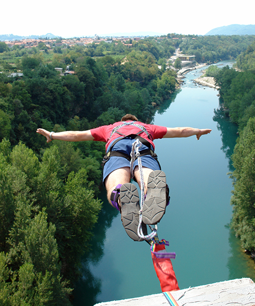
A man bungee jumping off a bridge

Example 5

Hollam made a bungee jump from a platform \(134\) m above a river. His height, in metres, during the first \(19\) seconds of his jump is shown in the table.

Time (s) \(0\) \(1\) \(2\) \(3\) \(4\) \(5\) \(6\) \(7\) \(8\) \(9\) \(10\) \(11\) \(12\) \(13\) \(14\) \(15\) \(16\) \(17\) \(18\) \(19\)
Height (m) \(134\) \(129\) \(117\) \(98\) \(72\) \(39\) \(24\) \(13\) \(9\) \(13\) \(24\) \(39\) \(54\) \(65\) \(69\) \(65\) \(54\) \(39\) \(24\) \(13\)
  1. Examine the data and select a suitable domain to model the data using a sinusoidal function. Justify your reasoning.
  2. Write a sinusoidal function to model Hollam's jump where \(h\left(t\right)\) is his height above the river in metres and \(t\) is the time in seconds after he begins his jump.

Solution — Part A

Here is a graph of Hollam's data:

The data from the table above are given in a scatter plot. The x-axis ranges from 0 to 20. The y-axis ranges from 0 to 160.

The first part of a bungee jump is free fall and is not influenced by the bungee cord.

From the data, Hollam's height decreases more slowly after \(5\) seconds which suggests that he was no longer free falling and the bungee cord was beginning to stretch.

We will use the domain \(\left\{ t\in\mathbb{R}\mid t\ge 5\right\}\) for our sinusoidal model. 

Solution — Part B

Hollam's minimum height was \(9\) m at \(8\) seconds and his maximum rebound height was \(69\) m at \(14\) seconds. This could be half of a sinusoidal cycle with an amplitude of \(\lvert a\rvert=\dfrac{69-9}{2}=30\) m and an average height of  \(k=\dfrac{69+9}{2}=39\) m. The period is \(2\left(14-8\right)=12\) seconds, so \(b=\dfrac{360}{12}=30\).

There are infinitely many functions that could model Hollam's height. Here are some sample functions.

The base sine function has a \(y\)-intercept on its axis and the function is increasing. If Hollam's function is 

  • a sine function, using the increasing axis point \(\left(11,39\right)\) then \(h=11\) and \(a\gt0\), \(h\left(t\right)=30\sin\left(30\left(t-11\right)\right)+39,~t\ge 5\);
  • a sine function, using the decreasing axis point \(\left(5,39\right)\) then \(h=5\) and \(a\lt0\), \(h\left(t\right)=-30\sin\left(30\left(t-5\right)\right)+39,~t\ge 5\).

The base cosine function has a \(y\)-intercept at its maximum, so if Hollam's function is

  • a cosine function, using the maximum point \(\left(14,69\right)\) then \(h=14\) and \(a\gt0\), \(h\left(t\right)=30\cos\left(30\left(t-14\right)\right)+39,~t\ge 5\);
  • a cosine function, using the minimum point \(\left(8,9\right)\) then \(h=8\) and \(a\lt0\), \(h\left(t\right)=-30\cos\left(30\left(t-8\right)\right)+39,~t\ge 5\).

Try This Revisited

The average daily temperatures for each month in Winnipeg, Manitoba, Canada are in the table below.

Month Jan Feb March April May June July Aug Sep Oct Nov Dec
High (\(^\circ\)C) \(-10\) \(-8\) \(0\) \(11\) \(17\) \(23\) \(26\) \(25\) \(20\) \(11\) \(2\) \(-8\)
Low (\(^\circ\)C) \(-18\) \(-17\) \(-9\) \(0\) \(7\) \(13\) \(16\) \(15\) \(10\) \(3\) \(-6\) \(-15\)
  1. Write sinusoidal functions to model the average daily high temperatures and the average daily low temperatures.
  2. Compare the properties of the functions. Describe why some properties are similar and others are different.

Solution — Part A

The outdoor temperature depends on the seasons so a sinusoidal model with a period of \(12\) months and \(b=\dfrac{360}{12}=30\) is reasonable.

Average Daily High Temperature

Let \(H\left(m\right)\) represent the average daily high temperature, in \(^\circ\)C, of month \(m\), where \(m=1\) is January and \(m=12\) is December.

From the data, the amplitude of the model sinusoidal function could be \(\dfrac{26-\left(-10\right)}{2}=18\).

The average daily high temperature for the year could be \(\dfrac{26+\left(-10\right)}{2}=8\).

The maximum of the data occurs in July, so a cosine function model could be \(H\left(m\right)=18\cos\left(30\left(m-7\right)\right)+8\).

Average Daily Low Temperature

Let \(L\left(m\right)\) represent the average daily low temperature, in \(^\circ\)C, of month \(m\).

The amplitude of the model sinusoidal function could be \(\dfrac{16-\left(-18\right)}{2}=17\).

The average daily low temperature for the year could be \(\dfrac{16+\left(-18\right)}{2}=-1\).

The maximum of the data occurs in July, so a cosine function model could be \(L\left(m\right)=17\cos\left(30\left(m-7\right)\right)-1\).

Solution — Part B

The amplitude, period, and phase shift of the two models are almost identical. This implies that when the daily high temperature is warmer, the daily low temperature is also warmer. This is reasonable as warmer days typically correspond to warmer nights as well.

The vertical translations for the models are different, \(+8\) compared to \(-1\). Since the rest of the model parameters are similar, the \(k\) values suggest that throughout the year, the daily highs are about \(8-\left(-1\right)=9^\circ\)C warmer than the daily lows. Looking at the data, we can see that differences between the highs and lows for each month is between \(7^\circ\) and \(10^\circ\). This is useful when you leave your home in the early afternoon and want to know whether or not you will need a jacket in the evening.

Angle of Elevation

When an object is sighted above an observer's horizontal plane, the angle between the observer's line of sight and the horizontal is called the angle of elevation.

The acute angle between a horizontal line and a line of sight is labelled

Example 6

SunPower Company is getting ready to install a solar panel with a device that controls the angle the panel rests on its post. The panel works most effectively if the sun's rays are perpendicular to the panel surface at noon each day. For the installation site, the angle of elevation of the sun at noon on selected days of the year is shown. Day \(1\) is Jan. 1st and day \(365\) is Dec. 31st.
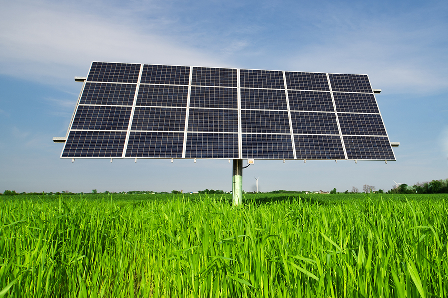
A large grid of solar panels

Day \(1\) \(31\) \(61\) \(91\) \(121\) \(151\) \(181\) \(211\) \(241\) \(271\) \(301\) \(331\) \(361\)
Angle (\(^\circ\)) \(53.8\) \(59.5\) \(67.2\) \(75.4\) \(83.2\) \(89.7\) \(91.3\) \(87.8\) \(79.0\) \(68.2\) \(58.3\) \(52.7\) \(53.2\)
  1. Write a sinusoidal function SunPower could use to keep the panel at the most effective angle each day.
  2. What angle of elevation will the panel be facing on March 21st?

Solution — Part A

  • We will assume we are modelling the angle of elevation for a non-leap year. If the function has a period of \(365\) days, then \(b=\dfrac{360}{365}=\dfrac{72}{73}\).
  • From the data, the maximum angle is \(91.3^\circ\) and the minimum angle is \(52.7^\circ\).
  • The amplitude for the model is \(\dfrac{91.3-52.7}{2}=19.3\) and \(k=\dfrac{91.3+52.7}{2}=72\).

Using a cosine function and the maximum data point \(\left(181,91.3\right)\), the model function is \(A\left(d\right)=19.3\cos\left(\dfrac{72}{73}\left(d-181\right)\right)+72\), where \(A\left(d\right)\) is the angle of elevation of the sun in degrees and \(d\) is the day of the year, day \(1\) is January 1st.

Alternatively, for a sine function model, we could use the increasing axis point one-quarter of the period or \(\dfrac{365}4=91.25\) days before the maximum at \(\left(89.75,72\right)\) so \(h=89.75\). The parameters \(a\), \(b\), and \(k\) would be the same as in previous cosine model, so the model function would be \(A\left(d\right)=19.3\sin\left(\dfrac{72}{73}\left(d-89.75\right)\right)+72\).

Solution — Part B

To determine the angle of elevation on March 21st, we need to determine the day number, and then evaluate the model function. Using the cosine model,

  • January has \(31\) days and February has \(28\) days, so March 21st is the \(80\)th day of the year.\[A\left(80\right)=19.3\cos\left(\dfrac{72}{73}\left(80-181\right)\right)+72\approx68.7759\]
  • On March 21st, the angle of elevation that the panel should be facing is approximately \(68.8^\circ\).

Check Your Understanding 2

Question — Version 1

A daily interest index for the term "math" on a search engine is the percent of the number of searches for "math" on a particular day compared to the highest number of searches for "math" in a day. The interest index for \(15\) consecutive days is shown.

Day \(1\) \(2\) \(3\) \(4\) \(5\) \(6\) \(7\) \(8\) \(9\) \(10\) \(11\) \(12\) \(13\) \(14\) \(15\)
Interest \(33\) \(34\) \(77\) \(88\) \(93\) \(98\) \(97\) \(34\) \(33\) \(39\) \(78\) \(85\) \(93\) \(99\) \(33\)

Identify the period to be used in a sinusoidal model of the data. Think about what the period reveals about the trend pattern of searches for "math" and why that pattern might exist.

Answer — Version 1

The period is \(7\) days.

Feedback — Version 1

There appears to be a weekly trend in the search interest. Days \(1\), \(8\), and \(15\) could be the beginning of the weekends when there might be less interest in school.

Therefore, a sinusoidal model of this data would have a period of \(7\) days.

Question — Version 2

The horizontal distance a swinging pendulum is from a wall is measured at various points in time. The resulting data is summarized in the following table: 

Time (s) \(0\) \(1\) \(2\) \(3\) \(4\) \(5\) \(6\) \(7\) \(8\) \(9\) \(10\) \(11\) \(12\) \(13\) \(14\)
Distance (cm) \(7.0\) \(8.5\) \(12.0\) \(15.5\) \(17.0\) \(15.5\) \(12.0\) \(8.5\) \(7.0\) \(8.5\) \(12.0\) \(15.5\) \(17.0\) \(15.5\) \(12.0\)

Identify the period to be used in a sinusoidal model of the data. Think about what the period tells you about the swinging pendulum.

Answer — Version 2

The period is \(8\) seconds.

Feedback — Version 2

The pendulum is closest to the wall at ‌\(0\) and ‌\(8\) seconds and furthest from the wall at ‌\(4\) and ‌\(12\) seconds.

Therefore, it takes \(8\) seconds for a complete swing of the pendulum, so a sinusoidal model of this data would have a period of \(8\) seconds.


Wrap-Up


Lesson Summary

  • Properties of sinusoidal functions can provide insight into the characteristics of real-world situations they model.
  • Data from real-world situations that demonstrate periodic behaviour can be used to determine the equations of sinusoidal models.

Take It With You

A double Ferris wheel is two rotating wheels attached to opposite ends of an arm that also rotates. The centres of the two wheels are \(18\) m apart. The arm is attached to the base of the wheel in the centre, \(15\) m above the ground, and the arm rotates clockwise at \(3\) revolutions per minute. Each of the two wheels has a radius of \(5\) m, and rotates clockwise at \(4\) revolutions per minute. The ride is \(12\) minutes long.

A double Ferris wheel

You board the ride at the bottom of a wheel when the arm is vertical.

  1. Sketch a graph of your height above the ground during the ride.
  2. Write an equation to model your height above the ground during the ride.