Graphing Five Base Functions Alternative Format
Lesson Part 1
Introduction
In any course involving the examination of functions and their general properties, it is necessary to develop tools to help us sketch the graphs of the functions. In order to do that, we require some basic graphs to work with.
In This Module
We will look at five base graphs.
- Quadratic function: \(f(x)=x^2\)
- Square root function: \(f(x)=\sqrt{x},\ \ x\ge 0\)
- Reciprocal function: \(f(x)=\dfrac{1}{x},\ \ x\neq 0\)
- Exponential function: \(f(x)=a^x,\ \ a\gt 0,\ \ a\neq 1\)
- Absolute value function: \(f(x)=\lvert x \rvert\)
For each of these functions, we will look at efficient ways to sketch their graph, discuss domain and range, and make observations about some characteristics or features of each graph.
For the exponential function, we will look at a specific case: \(f(x)=2^x\).
The Quadratic Function
Our first function is the quadratic function. This function is perhaps one that we are most familiar with.
Goal: Sketch the graph of \(f(x)=x^2\). State the domain and range. List any other features of the graph.
A common method for sketching any function is to use a table of values.
| \(x\) |
\(f(x)\) |
| \(-3\) |
\(9\) |
| \(-2\) |
\(4\) |
| \(-1\) |
\(1\) |
| \(0\) |
\(0\) |
| \(1\) |
\(1\) |
| \(2\) |
\(4\) |
| \(3\) |
\(9\) |
We could use any values for \(x\), but choosing convenient values is a good idea.
Plot the points and then join them with a smooth curve.
Since it is possible to square any real number, the domain is \(\{x \mid x \in \mathbb{R}\}\).
When any real number is squared, the result will be greater than or equal to \(0\).
Therefore, the range is \(\{y \mid y\ge 0, y \in \mathbb{R}\}\).
The graph is symmetric about the \(y\)-axis.
It has a minimum point which occurs at the vertex \((0,0)\).
The Square Root Function
Our second function to consider is the square root function.
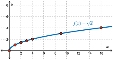
Goal: Sketch the graph of \(f(x)=\sqrt{x}\). State the domain and range. List any other features of the graph.
Give this example a try using a table of values approach.
| \(x\) |
\(f(x)\) |
| \(0\) |
\(0\) |
| \(1\) |
\(1\) |
| \(2\) |
\(1.41\) |
| \(3\) |
\(1.73\) |
| \(4\) |
\(2\) |
| \(9\) |
\(3\) |
| \(16\) |
\(4\) |
The square root of a negative number does not give a real number.
Thus, we use values for \(x\ge 0\).
We could choose any values for \(x \ge 0\), but generally choosing convenient values is a good idea.
Convenient values in this case would be values of \(x\), which have an integral square root. \(x = 0, 1, 4, 9, 16\) are five such values of \(x\) shown in the table of values.
Plot the points and then join them with a smooth curve.
Since the square root of a negative number does not give a real number, the domain is \(\{x \mid x \ge 0, x \in \mathbb{R}\}\).
The range is \(\{y \mid y\ge 0, y \in \mathbb{R}\}\).
The graph has a definite starting point at \((0,0)\).
The graph also appears to be related to the function \(y=x^2\).
This idea will be pursued in another module.
Lesson Part 2
The Reciprocal Function
The next function is the reciprocal function.
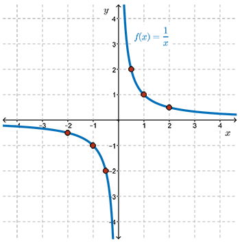
Goal: Sketch the graph of \(f(x)=\dfrac{1}{x}\). State the domain and range.
We will look at two methods for sketching this graph, but give it a try first.
The function takes a value of \(x\) and determines its reciprocal.
Only one value of \(x\), that is \(x=0\), would not be allowed since division by \(0\) is undefined.
We make a table of values as before and plot the points joining them with a smooth curve.
| \(x\) |
\(f(x)\) |
| \(-3\) |
\(-\frac{1}{3}\approx-0.3\) |
| \(-2\) |
\(-\frac{1}{2}=-0.5\) |
| \(-1\) |
\(-\frac{1}{1}=-1\) |
| \(0\) |
\(\frac{1}{0}\text{ is undefined}\) |
| \(1\) |
\(\frac{1}{1}=1\) |
| \(2\) |
\(\frac{1}{2}=0.5\) |
| \(3\) |
\(\frac{1}{3}\approx 0.3\) |
The final appearance of the graph is not entirely obvious.
It is not obvious what happens for values of \(x\), other than \(0\), between \(-1\) and \(1\).
Similarly, it is not obvious what happens to the function when \(x\) approaches positive or negative infinity.
The Reciprocal Function for \(-1\le x \le 1, x\not =0\)
As \(x\) gets closer and closer to \(0\) from the left side, the reciprocal approaches negative infinity.
We write this using the notation, “As \(x\rightarrow 0^-,\ \dfrac{1}{x}\rightarrow -\infty\).”
Similarly, as \(x\) gets closer and closer to \(0\) from the right side, the reciprocal approaches positive infinity.
We write this using the notation, “As \(x\rightarrow 0^+,\ \dfrac{1}{x}\rightarrow +\infty\).”
Some values are shown in the following tables of values.
| \(x\) |
\(f(x)\) |
| \(-1\) |
\(-1\) |
| \(-\frac{1}{2}\) |
\(-2\) |
| \(-\frac{1}{3}\) |
\(-3\) |
| \(\vdots\) |
\(\vdots\) |
| \(-\frac{1}{9}\) |
\(-9\) |
| \(-\frac{1}{10}\) |
\(-10\) |
| \(\vdots\) |
\(\vdots\) |
| \(-\frac{1}{1000}\) |
\(-1000\) |
| \(x\) |
\(f(x)\) |
| \(1\) |
\(1\) |
| \(\frac{1}{2}\) |
\(2\) |
| \(\frac{1}{3}\) |
\(3\) |
| \(\vdots\) |
\(\vdots\) |
| \(\frac{1}{9}\) |
\(9\) |
| \(\frac{1}{10}\) |
\(10\) |
| \(\vdots\) |
\(\vdots\) |
| \(\frac{1}{1000}\) |
\(1000\) |
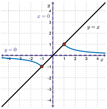
If you look at the graph and you see the values of \(x\) getting closer and closer to \(0\) from the right side of \(0\), you'll see that the graph gets closer and closer to the \(y\)-axis, but very, very large.
Similarly, as \(x\) goes from \(-1\) to \(0\) from the left side, the graph gets closer and closer to the \(y\)-axis again, but very large negative.
Note that the curve gets closer and closer to the \(y\)-axis but never crosses it.
The Reciprocal Function for \(x\le -1\) or \(x\ge 1\)
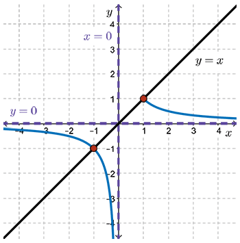
As \(x\) approaches negative infinity, the reciprocal gets closer to \(0\) and is negative.
We write this using the notation, “As \(x\rightarrow -\infty,\ \dfrac{1}{x}\rightarrow 0\) from below.”
Similarly, as \(x\) approaches positive infinity, the reciprocal gets closer and closer to \(0\) but stays positive.
We write this using the notation, “As \(x\rightarrow +\infty,\ \dfrac{1}{x}\rightarrow 0\) from above.”
Some values are shown in the following tables of values.
| \(x\) |
\(f(x)\) |
| \(-1\) |
\(-1\) |
| \(-2\) |
\(-\frac{1}{2}\) |
| \(-3\) |
\(-\frac{1}{3}\) |
| \(\vdots\) |
\(\vdots\) |
| \(-9\) |
\(-\frac{1}{9}\) |
| \(-10\) |
\(-\frac{1}{10}\) |
| \(\vdots\) |
\(\vdots\) |
| \(-1000\) |
\(-\frac{1}{1000}\) |
| \(x\) |
\(f(x)\) |
| \(1\) |
\(1\) |
| \(2\) |
\(\frac{1}{2}\) |
| \(3\) |
\(\frac{1}{3}\) |
| \(\vdots\) |
\(\vdots\) |
| \(9\) |
\(\frac{1}{9}\) |
| \(10\) |
\(\frac{1}{10}\) |
| \(\vdots\) |
\(\vdots\) |
| \(1000\) |
\(\frac{1}{1000}\) |
The curve gets closer and closer to the \(x\)-axis but never crosses it.
We will again discuss this a little bit later.
Lesson Part 3
The Reciprocal Function Summary
An asymptote is a line that the graph of a function approaches but does not touch for some values of \(x\) in the domain.
Some functions never touch an asymptote. But there are other functions which do. We will not pursue this second group of functions in this module.
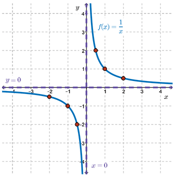
For the function \(f(x)=\dfrac{1}{x}\), there are two asymptotes.
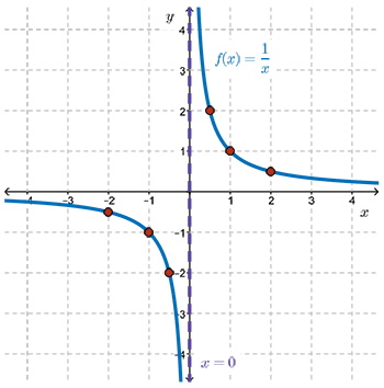
Since the graph approaches \(x=0\), the \(y\)-axis, but never touches it, \(x=0\) is a vertical asymptote.
Since the graph approaches \(y=0\), the \(x\)-axis, but never touches it, \(y=0\) is a horizontal asymptote.
Since \(f(x)=\dfrac{1}{x}\) never crosses the \(y\)-axis, the domain is \(\{x \mid x\not = 0,x\in \mathbb{R}\}\).
- We could also argue this by remembering that division by \(0\) is undefined.
Since \(f(x)=\dfrac{1}{x}\) never crosses the \(x\)-axis, the range is \(\{y \mid y\not = 0,y\in \mathbb{R}\}\).
We could argue this as follows.
- Move to any point on the \(y\)-axis other than the origin.
- Then by moving horizontally either to the left or to the right, we will intersect the graph at one point.
- That is, for every \(y\)-value, other than \(y=0\), there exists a point \((x,\ y)\) such that \(y=\dfrac{1}{x}\).
- However, there is no value of \(x\) in the domain such that \(\dfrac{1}{x}=0\).
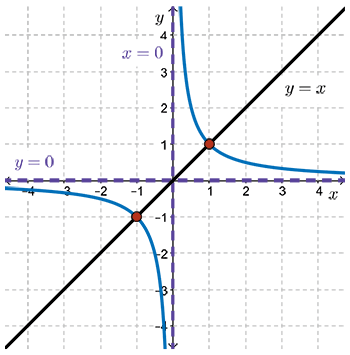
Asymptotes are generally shown using dashed lines.
The asymptotes, \(x=0\) and \(y=0\), are perpendicular to each other and intersect at the origin.
The complete graph is shown to the right.
Two lines, \(y=x\) and \(y=-x\), are also shown on the graph.
The function \(f(x)=\dfrac{1}{x}\) is symmetric about each of these lines.
Lesson Part 4
Another Way to Sketch the Reciprocal Function
There is another way to sketch the reciprocal function. And this method can be used to graph functions in a more general sense, and we'll describe that as we go.
Goal: Sketch the graph of \(f(x)=\dfrac{1}{x}\).
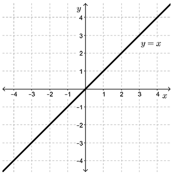
- Sketch the line \(y=x\). (In general, given \(f(x)=\dfrac{1}{g(x)}\), we graph the denominator function \(y=g(x)\).)
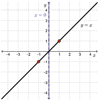
- When \(x=1\), \(\dfrac{1}{x}=1\). When \(x=-1\), \(\dfrac{1}{x}=-1\). The points \((1,1)\) and \((-1,-1)\) are on both \(y=x\) and \(y=\dfrac{1}{x}\).
Plot these two points. 
- Since \(x\not =0\), draw a vertical asymptote along the \(y\)-axis.
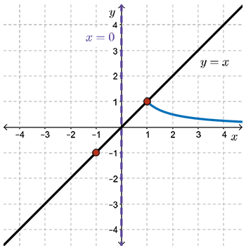
- As values of \(x\) go from \(1\) to \(+\infty\), \(\dfrac{1}{x}\) gets closer and closer to the positive \(x\)-axis from above.
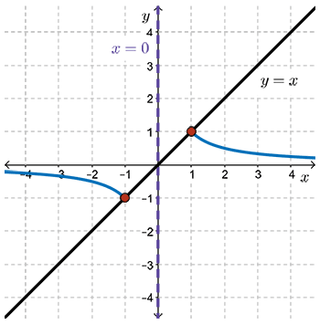
- As values of \(x\) go from \(-1\) to \(-\infty\), \(\dfrac{1}{x}\) gets closer and closer to the negative \(x\)-axis from below.
- Draw in the horizontal asymptote along the \(x\)-axis.
- As values of \(x\) go from \(-1\) to \(0\) from the left, \(\dfrac{1}{x}\) gets larger in a negative sense.
- As values of \(x\) go from \(1\) to \(0\) from the right, \(\dfrac{1}{x}\) gets larger in a positive sense.
So again we see this notion of a vertical asymptote, which we drew in a little bit earlier. Now we have the completed graph. This notion of graphing functions in this method will occur again in future modules in this course.
Lesson Part 5
The Exponential Function
The exponential function, in general, is written \(f(x)=a^x,\ a\gt 0,\ a\not = 1\).
For our purposes, we will graph a specific example: \(f(x)=2^x\).
Goal: Sketch the graph of \(f(x)=2^x\). State the domain and range. List any other features of the graph.
As before, we will use a table of values. Plot the points and then join them with a smooth curve.
| \(x\) |
\(f(x)=2^x\) |
| \(-4\) |
\(2^{-4}=\frac{1}{16}=0.0625\) |
| \(-3\) |
\(2^{-3}=\frac{1}{8}=0.125\) |
| \(-2\) |
\(2^{-2}=\frac{1}{4}=0.25\) |
| \(-1\) |
\(2^{-1}=\frac{1}{2}=0.5\) |
| \( 0\) |
\(2^{0}=1\) |
| \( 1\) |
\(2^{1}=2\) |
| \( 2\) |
\(2^{2}=4\) |
| \( 3\) |
\(2^{3}=8\) |
As \(x\) gets very large in a positive sense, \(2^x\rightarrow +\infty\).
We write this using the notation, “As \(x\rightarrow +\infty,2^x\rightarrow +\infty\).”
As \(x\) gets very large in a negative sense, \(2^x\rightarrow 0\) from above.
That is, the \(x\)-axis is a horizontal asymptote.
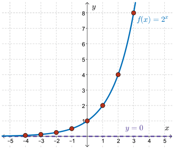
We write this using the notation, “As \(x\rightarrow -\infty,2^x\rightarrow 0\) from above.”
Since there is no value of \(x\) that cannot be used as the exponent, the domain is \(\{x \mid x\in \mathbb{R}\}\).
The graph is completely above the \(x\)-axis, so the range is \(\{y \mid y\gt 0,y\in \mathbb{R}\}\) and the horizontal asymptote is \(y=0\), the \(x\)-axis.
For this next function, some students will not be familiar with this function. So we'll start with the definition.
The Absolute Value Function
The absolute value of any real number \(x\), written \(\lvert x \rvert\), is the numeric value of \(x\) without regard to its sign.
Geometrically, \(\lvert x \rvert\) can be thought of as the distance from \(x\) to \(0\) on the real number line, without regard to direction.
Using function notation, we write
\[ f(x)=\begin{cases} x, & \text{if } x \ge0 \\-x, & \text{if } x \lt 0 \end{cases} \]
When \(x=5\), \(f(5)=5\).
When \(x=-3\), \(f(-3)=-(-3)=3\).
And when \(x=0\), \(f(0)=0\).
Goal: Sketch the graph of \(f(x)=\lvert x \rvert\). State the domain and range. List any other features of the graph.
To graph \(f(x)=\lvert x \rvert\), we will construct a table of values and then plot the points before joining them.
| \(x\) |
\(f(x)=\lvert x \rvert \) |
| \(-3\) |
\(3\) |
| \(-2\) |
\(2\) |
| \(-1\) |
\(1\) |
| \( 0\) |
\(0\) |
| \( 1\) |
\(1\) |
| \( 2\) |
\(2\) |
| \(3\) |
\(3\) |
The graph of \(f(x)=\lvert x \rvert\) looks like the letter “V.”
We can find the absolute value of any value of \(x\) so the domain is \(\{x \mid x\in \mathbb{R}\}\).
The minimum point on the graph is the origin so the range is \(\{y \mid y\ge0,y\in \mathbb{R}\}\).
The graph is symmetric about the \(y\)-axis.
Summary
We have looked at five base graphs.
Each graph has a distinctive shape and key features.
You should familiarize yourself with efficient ways to sketch each base graph.
You should familiarize yourself with the domain, range, and key features of each function.