Applications with the Sine and Cosine Functions Alternative Format

Lesson Part 1

Introduction

In this module we are going to take a look at applications which can be modelled using sinusoidal functions. Through earlier studies in mathematics, a variety of functions have been used to model specific applications.

For example, the relationship between a worker's pay and the number of hours worked could be modelled with a simple linear function.

When a ball is thrown into the air, its height above the ground over time can be modelled using a quadratic function.

Growth and decay situations can be modelled with exponential functions.

In this module, sine and cosine functions will be used to model various physical situations that are periodic.

Examples

Example 1

The pendulum of an antique clock makes \(30\) complete swings in one minute. A complete swing moves the pendulum from the extreme right point, \(R\), to the extreme left point, \(L\), and back to \(R\) again. The horizontal distance between the two extreme points \(R\) and \(L\) is \(36\) cm.

Example 1 — Part A

a. Determine the period and amplitude of this motion.

Solution

Since there are \(30\) complete swings in \(60\) seconds (or \(1\) minute), \(1\) period is \(60 \div 30 = 2\) seconds.

The horizontal distance between the two extreme points is \(36\) cm. That is, the maximum minus the minimum is \(36\).

The amplitude is half of this value, so the amplitude is \(18\).

Example 1 — Part B

b.Draw a sketch to model the pendulum swing for the first \(6\) seconds. Assume the pendulum starts at \(R\).

Solution

Let \(d\) represent the horizontal distance from \(\color{Mulberry}M\), with positive distance to the right and negative distance to the left. When the pendulum is at \(\color{NavyBlue}R\), \(d=18\). When the pendulum is at \(\color{BrickRed}L\), \(d=-18\).

Since the period is \(2\) seconds, the pendulum will be at \(\color{NavyBlue}R\) (we'll consider that a maximum) at \(0\), \(2\), \(4\), and \(6\) seconds.

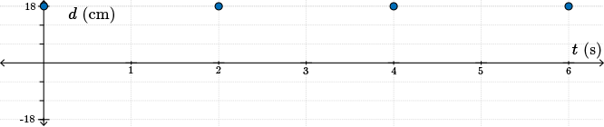
The minimum will occur at the halfway point of each period, so the pendulum will be at \(\color{BrickRed} L\) at \(1\), \(3\), and \(5\) seconds.

And halfway between the maximum and minimum, the pendulum will be at \(\color{Mulberry}M\). The pendulum, therefore, will be at \(\color{Mulberry}M\) at \(0.5\), \(1.5\), \(2.5\), \(3.5\), \(4.5\), and \(5.5\) seconds.

A sketch is shown.

Example 1 — Part C

c. Determine an equation to model the path of the pendulum.

Solution

By referring to the sketch, it would appear that the path of the pendulum can be modelled using a cosine function, whose general equation is 

\[ d = a\cos[b(x-h)]+k\] 

Since a maximum point on the sketch is on the \(y\)-axis (or in this case, the \(d\)-axis), there is no horizontal translation and so \(h=0\).

The central horizontal axis is on the \(x\)-axis (or in this case, the \(t\)-axis) so there is no vertical translation and \(k=0\).

The amplitude is \(18\) cm. Since a maximum point is on the positive \(y\)-axis, there has been no reflection about the \(x\)-axis and \(a=18\).

The period is \(2\) seconds. Thus, \(b = \dfrac{2\pi}{\text{period}} = \dfrac{2\pi}{2} = \pi\).

Substituting for \(a=18\), \(b=\pi\), \(h=0\), and \(k=0\) into our general equation for the cosine function, \(d=a\cos[b(x-h)]+k\), we obtain \(d=18\cos(\pi x)\).

If we use \(t\) instead of \(x\), an equation of the function graphed becomes \(d=18\cos(\pi t)\), and again the restriction we've set is \(0\leq t \leq 6\).

• When \(d \lt 0\), the pendulum is closer to \(\color{BrickRed}L\) than it is to \(\color{NavyBlue}R\).
• When \(d \gt 0\), the pendulum is closer to \(\color{NavyBlue}R\) than it is to \(\color{BrickRed}L\).
• When \(d=0\), the pendulum is at \(\color{Mulberry}M\).

Once we have a model, we can use it to determine other things.

Example 1 — Part D

d. Using the model, determine the position of the pendulum at \(4.75\) seconds.

Solution

Substitute \(t=4.75\) into our equation \(d=18\cos(\pi t)\):

\[ \begin{align*} d &= 18\cos(4.75\pi) \\ &= 18\cos \left ( \dfrac{19\pi}{4}\right) &&\text{converting to an equivalent fraction}\\ &= 18\cos\left(\dfrac{3\pi}{4}\right) &&\text{since }\dfrac{19\pi}{4} \text{ and }\dfrac{3\pi}{4} \text{ are coterminal angles} \\ &= 18\left ( \dfrac{-1}{\sqrt{2}}\right ) \\ &= 18 \left (\dfrac{-1}{\sqrt{2}}\right ) \times \left ( \dfrac{\sqrt{2}}{\sqrt{2}}\right ) \\ &= -9\sqrt{2} \end{align*} \]

At \(t=4.75\), the pendulum is located \(9\sqrt{2}\) cm to the left of the middle position, closer to \(L\) than to \(R\).

We can use the sketch to see that our calculation is reliable.

And indeed it is.

This is a good time to note that the motion of the pendulum is only approximately sinusoidal. The exact motion of the pendulum would be studied in university physics or applied mathematics courses.

Example 1 — Part E

e. At what times during the first \(6\) seconds will the pendulum be horizontally \(9\) cm to the right of its position at \(M\)?

Solution

Substitute \(9\) for \(d\) into our equation, \(d=18\cos(\pi t)\):

\[ \begin{align*} 9 &= 18\cos(\pi t) \\ \tfrac{1}{2} &= \cos(\pi t) \end{align*} \]

In an earlier module we made a substitution. And we'll do the same here. Let \(\theta=\pi t\). We want \(\cos(\theta)=\frac{1}{2}\).

Well, we know from our work that The reference angle is \(\frac{\pi}{3}\). And we also know that since \(\cos(\theta)\gt 0\), \(\theta\) is in quadrant 1 or in quadrant 4.

In quadrant 1, \(\theta = \frac{\pi}{3}\) and in quadrant 4, \(\theta=2\pi - \frac{\pi}{3} = \frac{5\pi}{3}\). Those are the answers for \(0\leq\theta\leq 2\pi\).

Since \(\theta = \pi t\), we can substitute back and solve for \(t\) by dividing by \(\pi\):

These two possibilities for \(t\) lie in the interval \(0 \leq t \leq 2\).

To get all times such that \(0\leq t \leq 6\), add multiples of the period length. It follows that the pendulum will be horizontally \(9\) cm to the right of its position at \(M\) for \(t=\frac{1}{3}, 1\frac{2}{3}, 2\frac{1}{3}, 3\frac{2}{3},4\frac{1}{3},5\frac{2}{3}\) seconds.

Lesson Part 2

The Ferris Wheel

As the module goes forward, we will consider the periodic nature of a ride on the ferris wheel.

The Ferris wheel is a ride often found at exhibitions or fairs.

Riders enter and exit the ride at the same point. The circular ride takes its passengers through several revolutions at a constant speed. Our interest in this type of amusement ride is its periodic nature.

We can model this situation with a sinusoidal function which relates the rider's height above the ground to the length of time on the ride.

Use the worksheet to make connections between various elements of a Ferris wheel ride and features of sinusoidal functions such as period, amplitude, and phase shift.

Investigation

See the investigation in the side navigation.

Lesson Part 3

Examples

Example 2

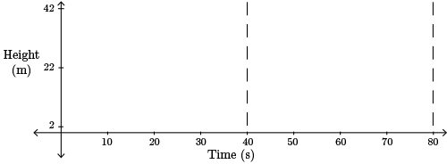
A Ferris wheel with a radius of \(20\) m makes one complete revolution every \(40\) s. The rider's initial position on the ride is at the bottom of the wheel, \(2\) m above the ground.

Example 2 — Part A

a. Draw a graph showing a rider's height above the ground during the first two revolutions of the wheel.

Solution

Since one revolution takes \(40\) s, the period length is \(40\) s.

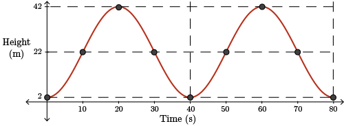
The rider gets on at the lowest point so a minimum occurs at \((0,2)\). Minimums also occur at \((40,2)\) and \((80,2)\) since each complete revolution takes \(40\) s.

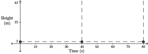
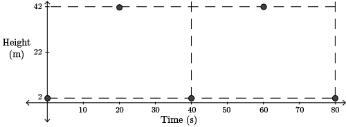
The rider gets on at a point \(2\) m above the ground. The Ferris wheel has a radius of \(20\) m or, in fact, a diameter of \(40\) m. So, the maximum height above the ground is \(2+40\) or \(42\) m.

Maximums occur half of a period after each minimum. Therefore, maximums occur at \((20,42)\) and \((60,42)\).

The centre of the wheel is at \(2+20\) (\(2\) m above the ground and \(20\) m radius) or \(22\) m above the ground. The rider is at this height at any time that is halfway between the times when adjacent maximum and minimum heights occur.

Therefore, the rider is \(22\) m above the ground at \(10\) s, \(30\) s, \(50\) s, and \(70\) s.

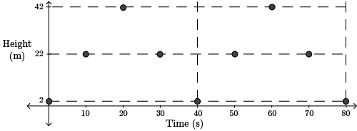
A final sketch is shown.

Example 2 — Part B

b. Determine an equation modelling the rider's height above the ground during the first two minutes of the ride.

Solution

Let's extend our sketch to \(120\) seconds (or \(2\) minutes).

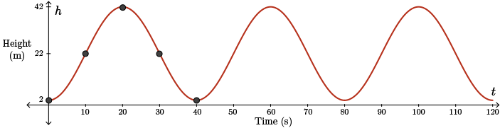
To keep things simpler, we will model with the negative cosine function since the phase shift will be \(0\). If you look at the sketch, you can see five points are shown on the graph.

Since the amplitude is \(20\), let \(a=-20\).

The middle height is \(22\) m so the central horizontal axis is at \(y=22\) and it follows that \(k=22\).

The period is \(40\) so \(b=\dfrac{2\pi}{40} = \dfrac{\pi}{20}\).

Therefore, an equation to model this situation is \(y=-20\cos\left (\dfrac{\pi}{20}x\right)+22\).

Using variables, which are more representative of the situation, we can write the equation as

\[h=-20\cos\left(\dfrac{\pi}{20}t\right)+22\]

for \(0\leq t \leq 120\), where \(h\) is the rider's height, in metres, above the ground at time \(t\) seconds.

Check Your Understanding A

This question is not included in the Alternative Format, but can be accessed in the Review section of the side navigation.

Example 2 — Part C

So now we have our model, or we have a model, and we'd like to answer the following question.

c. At what times during the first two minutes will the rider's height above the ground be \(38\)m or higher?

Solution

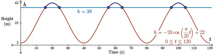
To help us visualize this, draw the horizontal line \(\color{NavyBlue}h=38\) on the graph.

We want to determine the times when the sinusoidal function intersects the line and when it is above the line.

Let \(A=\frac{\pi}{20}t\) and \(h=38\). Then our equation becomes

\[ \begin{align*} 38 &=-20\cos(A)+22 \\ 16 &=-20\cos(A) \\ -\tfrac{4}{5} &= \cos(A) \end{align*} \]

The reference angle, in radians, is \(\cos^{-1}\left(-\frac{4}{5}\right) = \cos^{-1} (0.8) \approx 0.644\), rounded to three decimal places.

Since \(\cos(A)\lt 0\), \(A\) is in quadrant 2 or quadrant 3.

In quadrant 2, \(A=\pi-\cos^{-1}\left ( \frac{4}{5}\right ) \approx 2.498\) and in quadrant 3, \(A=\pi + \cos^{-1}\left ( \frac{4}{5}\right ) \approx 3.785\).

But \(A=\frac{\pi}{20}t\), so as we did earlier, we're going to solve two equations for the approximate values of \(t\). So we have

\[ \begin{align*} \tfrac{\pi}{20}t &= 2.498 \\ t &= \tfrac{2.498\times 20}{\pi} \\ &\approx 15.9~\text{s} \end{align*} \]

and 

\[ \begin{align*} \tfrac{\pi}{20}t &= 3.785 \\ t &= \tfrac{3.785\times 20}{\pi} \\ &\approx 24.1~\text{s} \end{align*} \]So if you look at our sketch, the rider is \(38\) m or higher above the ground for \(15.9 \leq t \leq 24.1\).

Looking back at the graph, this is the first section where the sinusoidal function is on or above the line \(\color{NavyBlue} h=38\).

To get the other two intervals, simply add multiples of the period, \(40\) seconds, to each endpoint of the first interval.

In the first \(120\) seconds, the rider is \(38\) m or higher above the ground from \(15.9\) s to \(24.1\) s, from \(55.9\) s to \(64.1\) s, and from \(95.9\) s to \(104.1\) s.

Check Your Understanding B

This question is not included in the Alternative Format, but can be accessed in the Review section of the side navigation.

Lesson Part 4

Examples

In this next example, we're going to look at some data.

Example 3

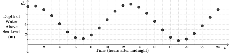
Saint John, New Brunswick, Canada is located on the Bay of Fundy. The depth of the water above sea level is affected by the ocean tides. The following chart gives the depth of the water over a \(24\)-hour period in early December.

Hours after Midnight	\(0\)	\(1\)	\(2\)	\(3\)	\(4\)	\(5\)	\(6\)	\(7\)	\(8\)	\(9\)	\(10\)	\(11\)	\(12\)
Water Depth (m)	\(7.5\)	\(7.6\)	\(6.9\)	\(5.7\)	\(4.1\)	\(2.5\)	\(1.4\)	\(1.2\)	\(1.9\)	\(3.2\)	\(4.9\)	\(6.6\)	\(7.7\)

Hours after Midnight	\(13\)	\(14\)	\(15\)	\(16\)	\(17\)	\(18\)	\(19\)	\(20\)	\(21\)	\(22\)	\(23\)	\(24\)
Water Depth (m)	\(8.0\)	\(7.4\)	\(6.2\)	\(4.6\)	\(2.9\)	\(1.4\)	\(0.8\)	\(1.1\)	\(2.2\)	\(3.7\)	\(5.4\)	\(6.9\)

Fisheries and Oceans Canada (2014). Saint John (#65). Retrieved from http://tides.gc.ca/eng/station?sid=65 on December 8, 2014.

Example 3 — Part A

a. Draw a graph showing the water depth versus time over the \(24\)-hour period.

Solution

Our sketch is shown.

Example 3 — Part B

b. Estimate the maximum and minimum depths over the \(24\)-hour period. Use these values to estimate the mean (average) depth of the water and then approximate the values for the amplitude and vertical displacement to be used in a sinusoidal model.

Solution

From the data, the maximum depth of the water is \(8.0\) m occurring \(13\) hours after midnight.

The minimum depth of the water is \(0.8\) m occurring \(19\) hours after midnight.

Using these maximum and minimum depths, the mean depth of the water is the average of those two, \(\dfrac{0.8+8.0}{2}=4.4\) m. This new information is now shown on our sketch.

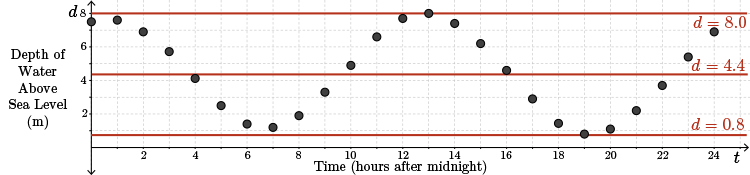
We can now approximate the amplitude and the vertical displacement.

The amplitude is the maximum value subtract the minimum value divided by \(2\), or \(a=\dfrac{8.0-0.8}{2}=3.6\) and the vertical displacement is \(k=4.4\).

Example 3 — Part C

c. From the graph, we see that the function appears to be periodic. Estimate the period length.

Solution

There are many ways to arrive at an estimate for the period.

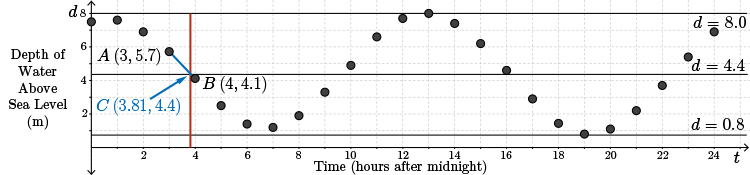
Looking at the horizontal distance between the two maxima and the two minima, the period is close to \(12\) hours.

However, it is known that the period of the tides is between \(12\) and \(13\) hours. So, we will refine our estimate.

One way to do this is to draw a line segment connecting the point corresponding to the depth of the water at 3 hours, \(A~(3,5.7)\), to the point corresponding to the depth of the water at 4 hours, \(B~(4,4.1)\). This line segment intersects the central horizontal axis.

We could determine the intersection by finding the equation of the line passing through \(A\) and \(B\). Then, we would find the point where this line crosses the line \(y=4.4\). This will be left as an exercise for you to pursue.

This intersection point, labeled \(C\) on the graph, is approximately \((3.81, 4.4)\).

If we connect the points \(D~(16,4.6)\) and \(E~(17,2.9)\), this line segment intersects the central horizontal axis at approximately \(F~(16.12,4.4)\).

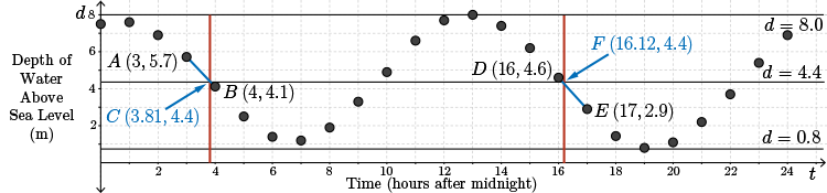
An estimate for the period is calculated as the difference between the \(x\)-coordinate of \(F\) and the \(x\)-coordinate of \(C\).

The length of the period is \(16.12-3.81=12.31\) hours or about \(12\) hours and \(19\) minutes.

Example 3 — Part D

d. Determine an equation to model the depth, \(d\), of the water versus time, \(t\), over the \(24\)-hour period.

Solution

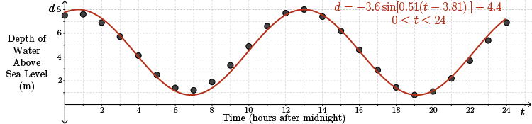
From earlier work with this example, we found that the amplitude was approximately \(3.6\) and the vertical displacement was \(4.4\).

Since the period length is \(12.31\), \(b=\dfrac{2\pi}{12.31}\approx 0.51\).

If we use \(C~(3.81,4.4)\) as the first point of a five-point sketch, then the phase shift is \(3.81\) and so \(h=3.81\). We will model with a sine function that has been reflected about the \(t\)-axis but not about the \(d\)-axis.

It follows that \(a=-3.6\) and \(b=0.51\).

Combining all of the information and substituting into the general equation for the sine function, \(d=a\sin[b(t-h)]+k\), we obtain

\[d=-3.6\sin[0.51(t-3.81)]+4.4, ~~0\leq t \leq 24\]

Check Your Understanding C

This question is not included in the Alternative Format, but can be accessed in the Review section of the side navigation.

Solution Continued

Our model has been added to the plot of the points. We see that our model is reasonably close.

We could also have obtained an equation to model this \(24\)-hour period using the sinusoidal regression function available on most graphing calculators.

Example 3 — Part E

e. If a ship requires a minimum of \(5\) m of water to safely enter the harbour, on this particular day, determine the times in the \(24\)-hour period when it is safe for the ship to enter.

Solution

We want the times when the curve is on or above the line \(\color{NavyBlue} d=5\). The times can be estimated from the graph or determined algebraically.

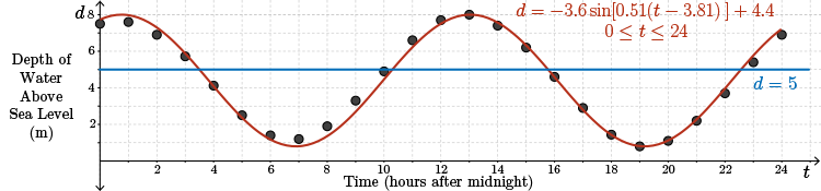
Looking at the graph, we estimate that the ship can come into the harbour from midnight to 3:30 AM, from 10:30 AM to 3:30 PM, and from 10:30 PM to midnight.

Algebraically, let \(d=5\) and let \(\theta=0.51(t-3.81)\) in

\[d=-3.6[0.51(t-3.81)]+4.4\]

Now, solve the equation \(5=-3.6\sin(\theta)+4.4\).

Simplifying, \(\sin(\theta) = - \dfrac{0.6}{3.6}=-\dfrac{1}{6}\).

The reference angle is \(\sin^{-1}\left (\dfrac{1}{6}\right) \approx 0.1674\) radians. Since \(\sin(\theta)\lt 0\), \(\theta\) is in quadrant 3 or quadrant 4.

In quadrant 3, we know how to calculate \(\theta\), \(\theta = \pi+\sin^{-1} \left (\dfrac{1}{6}\right )\approx 3.3090\) and in quadrant 4, \(\theta =2\pi-\sin^{-1}\left ( \dfrac{1}{6}\right ) \approx 6.1157\).

Substituting \(\theta = 0.51(t-3.81)\) in our equation again and solving for two possible answers for \(t\) we have

\[ \begin{align*} 0.51(t-3.81) &=3.3090 \\ t &=\dfrac{3.3090}{0.51} + 3.81 \\ t &\approx 10.30 \text{h} \end{align*} \]

or 

\[ \begin{align*} 0.51(t-3.81) &= 6.1157 \\ t &=\dfrac{6.1157}{0.51} +3.81 \\ t &\approx 15.80 \text{h} \end{align*} \]

We want all possible values for \(t\) such that \(0\leq t \leq 24\) so we need to determine all possible coterminal angles in this interval.

The period is \(12.31\), so other possible values for \(t\) are \(10.3+12.31=22.61\) and \(15.80-12.31=3.49\). Adding or subtracting other multiples of the period will produce values outside the required domain.

The depth of the water is \(5\) m when \(t=3.49\) h, \(t=10.30\) h, \(t=15.80\) h, or \(t=22.61\) h. Converting these to more recognizable times, the depth is \(5\) m at 3:29 AM, at 10:18 AM, at 3:48 PM, and at 10:37 PM.

Using these times in combination with the graph, the ship can enter the harbour safely from midnight to 3:29 AM, from 10:18 AM to 3:48 PM, and from 10:37 PM to midnight.

Check Your Understanding D

This question is not included in the Alternative Format, but can be accessed in the Review section of the side navigation.

Summary

There are many real world applications which are periodic that can be modelled using the sine or cosine functions. In this module, we have attempted to illustrate a few of these examples and solve related problems.

Changing Depths of Water Due to Tidal Influence