Moving from Secants to Tangents Alternative Format
Lesson Part 1
Introduction
In previous modules, recall that we discussed the following:
A secant intersects a curve in at least two distinct points.
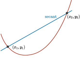
The slope of the secant represents the average rate of change of the function over an interval.
A tangent touches a curve at one point.
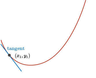
It does not cross the curve at that point if extended. A tangent most resembles the curve near that point.
The slope of the tangent represents the instantaneous rate of change of the function at that point.
In this module, we will develop an algebraic method using limits to find the slope of a tangent to a curve.
That is, we will develop a method for determining the instantaneous rate of change of a function at a point.
Approximating the Slope of a Tangent to a Curve
Example 1
Find the slope of the tangent to the parabola \(f(x) = x^2\) at the point \(P\,(3,9)\).
Solution
When using the slope formula \(m = \dfrac{y_{2} - y_{1}}{x_{2} - x_{1}}\), two ordered pairs are required.
The tangent only has one known ordered pair: the point of tangency.
We need to determine another point on \(f(x) = x^2\) “close” to the point of tangency.
Let \(Q\) be a point on \(f(x) = x^2\), close to \(P\), with \(x\)-coordinate \(3 + \Delta x\).
Then, \(f(3 + \Delta x) = (3 + \Delta x)^2\).
We will let the values of \(\Delta x\) get closer and closer to zero so that the point \(Q\) gets closer and closer to the point of tangency, \(P\).
Part 1: For \(\Delta x = 0.1\), determine the coordinates of \(Q\) and the slope of the secant \(PQ\).
For \(\Delta x = 0.1\), the \(x\)-coordinate of point \(Q\) is \(x = 3 + 0.1 = 3.1\), and \(f(3.1) = 3.1^2 = 9.61\).
So, the point \(Q\) has the coordinate \((3.1, 9.61)\).
We can calculate the slope of the secant \(PQ\):
\[ \begin{align*} m_{PQ} &= \dfrac{\Delta y}{\Delta x} \\ &= \dfrac{f(3.1) - f(3)}{3.1 - 3} \\ &= \dfrac{9.61 - 9}{0.1} \\ &= 6.1 \end{align*} \]
Part 2: For \(\Delta x = 0.001\), determine the coordinates of \(Q\) and the slope of the secant \(PQ\).
For \(\Delta x = 0.001\), the \(x\)-coordinate of point \(Q\) is \(x = 3 + 0.001 = 3.001\), and \(f(3.001) = 3.001^2 = 9.006001\).
So, the point \(Q\) has the coordinate \((3.001, 9.006001)\).
We can calculate the slope of the secant \(PQ\):
\[ \begin{align*} m_{PQ} &= \dfrac{\Delta y}{\Delta x} \\ &= \dfrac{f(3.001) - f(3)}{3.001 - 3} \\ &= \dfrac{9.006001 - 9}{0.001} \\ &= 6.001 \end{align*} \]
Part 3: For \(\Delta x = -0.001\), determine the coordinates of \(Q\) and the slope of the secant \(PQ\).
For \(\Delta x = -0.001\), the \(x\)-coordinate of point \(Q\) is \(x = 3 - 0.001 = 2.999\), and \(f(2.999) = 2.999^2 = 8.994001\).
So, the point \(Q\) has the coordinate \((2.999, 8.994001)\).
We can calculate slope of the secant \(PQ\):
\[ \begin{align*} m_{PQ} &= \dfrac{\Delta y}{\Delta x} \\ &= \dfrac{f(2.999) - f(3)}{2.999 - 3} \\ &= \dfrac{8.994001 - 9}{-0.001} \\ &= 5.999 \end{align*} \]
Part 4: The following table contains results found by using different values of \(\Delta x\). Three of the slopes were calculated in this example.
| \(\Delta x\) |
Coordinates of \(Q\) |
Slope of \(PQ\) |
\(\Delta x\) |
Coordinates of \(Q\) |
Slope of \(PQ\) |
| \(0.1\) |
\((3.1, 9.61)\) |
\(6.1\) |
\(- 0.1\) |
\((2.9, 8.41)\) |
\(5.9\) |
| \(0.01\) |
\((3.01, 9.0601)\) |
\(6.01\) |
\(-0.01\) |
\((2.99, 8.9401)\) |
\(5.99\) |
| \(0.001\) |
\((3.001, 9.006001)\) |
\(6.001\) |
\(-0.001\) |
\((2.999, 8.994001)\) |
\(5.999\) |
Using the values in the table, predict the slope of the tangent to the parabola \(f(x) = x^2\) at the point \(P\,(3,9)\).
If you look at the right three columns of the table, as \(Q\) gets closer and closer to \(P\), approaching from the left, the slope of the secant gets closer and closer to \(6\), approaching from below.
As \(Q\) gets closer and closer to \(P\), approaching from the right, the slope of the secant gets closer and closer to \(6\), approaching from above.
It would be reasonable to say that the slope of the tangent at \(P\,(3,9)\) is \(6\).
Lesson Part 2
Using Limits to Determine the Slope of a Tangent to a Curve
In the last example, we estimated the slope of the tangent at \(x = 3\) to be \(6\) by determining what the slope of the secant approaches as \(\Delta x\) approaches \(0\).
That is, as \(\Delta x \rightarrow 0\), the slope of the secant \(\dfrac{f(3 + \Delta x) - f(3)}{(3 + \Delta x) - 3} = \dfrac{f(3 + \Delta x) - f(3)}{\Delta x} \rightarrow 6\).
The concept of a limit was introduced earlier in the Rational Functions unit, and it was used to describe the behaviour of the graph of a function about its asymptotes as well as its end behaviour.
We can use limits in this situation to communicate our findings concerning the slope of the tangent to a function at a point.
A limit provides information about how a function behaves near, not at, a specific value of \(x\).
If the limit of a function \(y = f(x)\) as \(x\) approaches \(a\) is equal to \(L\), then we write
\[{\color{BrickRed}\displaystyle\lim_{x \rightarrow a} f(x) = L}\]
We read this as, “the limit as \(x\) approaches \(a\) of \(f(x)\) equals \(L\).”
This means that \(f(x)\) gets closer and closer to the value \(L\) as \(x\) gets closer and closer to the value \(a\).
That is, \(y \rightarrow L\) as \(x \rightarrow a\).
In this situation, we determined that
\[\dfrac{f(3 + \Delta x) - f(3)}{\Delta x} \rightarrow 6 \ \text{as} \ \Delta x \rightarrow 0\]
Thus, using limits and limit notation, the slope of the tangent at \(x = 3\) is given by
\[m_{\text{tangent}} = \displaystyle\lim_{\Delta x \rightarrow 0} \dfrac{f(3 + \Delta x) - f(3)}{(3 + \Delta x) - 3} = 6\]
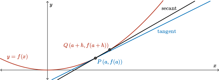
Generalizing the example, let \(Q\) be a point on \(f(x) = x^{2}\) close to \(P\,(3, 9)\).
The coordinates for \(Q\) are \((3 + h, f(3 + h))\), where \(h\) is extremely close to zero.
The slope of the tangent \(P\) is given by the general formula
\[ m_{\text{tangent}} = \displaystyle\lim_{\Delta x \rightarrow 0} \dfrac{\Delta y}{\Delta x} \]
Substituting for \(\Delta x\) and \(\Delta y\), we get
\[ m_{\text{tangent}}= \displaystyle\lim_{h \rightarrow 0} \dfrac{f(3 + h) - f(3)}{(3+h) - 3} \]
Then, if we substitute the values of \(f(3+h)\) and \(f(3)\), we get the expression
\[ m_{\text{tangent}}= \displaystyle\lim_{h \rightarrow 0} \dfrac{(3+h)^2 - 9}{h} \]
We then expand the numerator:
\[ m_{\text{tangent}}= \displaystyle\lim_{h \rightarrow 0} \dfrac{9 + 6h + h^2 - 9}{h} \]
Simplify the numerator, we get
\[ m_{\text{tangent}}= \displaystyle\lim_{h \rightarrow 0} \dfrac{6h + h^2}{h} \]
Then, common factoring the numerator, we get
\[ m_{\text{tangent}}= \displaystyle\lim_{h \rightarrow 0} \dfrac{h(6+h)}{h} \]
Since \(h\neq 0\), we can divide out the \(h\) in the numerator and the denominator:
\[ \begin{align*} m_{\text{tangent}} &= \displaystyle\lim_{h \rightarrow 0} \dfrac{\cancel{h}(6+h)}{\cancel{h}} \\ &= \displaystyle\lim_{h \rightarrow 0} (6 + h) \end{align*} \]
Then, we can simply evaluate by substituting \(h=0\):
\[ m_{\text{tangent}}= 6 \]
This is the value of the slope that we got before.
In general, the slope of a tangent to a function (instantaneous rate of change) is defined by
\[m_{\text{tangent}} = \displaystyle\lim_{\Delta x \rightarrow 0} \dfrac{\Delta y}{\Delta x}\]
To determine the slope of the tangent to \(y = f(x)\) at \(x = a\), we can use
\[ \begin{align*} m_{\text{tangent}} \big\vert_{x = a} &= \displaystyle\lim_{h \rightarrow 0} \dfrac{f(a + h) - f(a)}{(a+h) - a} \\ &= \displaystyle\lim_{h \rightarrow 0} \dfrac{f(a + h) - f(a)}{h}, \quad \Delta x = h \end{align*} \]
You will learn much more about limits in the study of calculus.
For now, we will use limit notation to communicate the procedure used when determining the instantaneous rate of change or the slope of a tangent. Limit notation will help distinguish this procedure from the method used to determine average rate of change or slope of a secant.
Lesson Part 3
Finding the Equation of a Tangent
Example 2 — Part A
Given the function \(f(x) = x^2 + 3x\):
Find the slope of the tangent at \(P\,(2,10)\).
Solution
Find the \(y\)-coordinates of the points on the curve with \(x\)-coordinates \(2\) and \(2 + h\).
\[ \begin{align*} f(2) &= 10 \\ f(2+h) &= (2+h)^2 + 3(2 + h) \\ &= 4 + 4h + h^2 + 6 + 3h \\ &= h^2 + 7h + 10 \end{align*} \]
Now, we go through the procedure to find the slope of the tangent at point \(P\):
\[ m = \displaystyle\lim_{h \rightarrow 0} \dfrac{f(2 + h) - f(2)}{(2+h)-2} \]
Substituting for \(f(2 + h)\) and \(f(2)\),
\[ m = \displaystyle\lim_{h \rightarrow 0} \dfrac{h^2 + 7h + 10 - 10}{h} \]
Simplifying the numerator,
\[ m = \displaystyle\lim_{h \rightarrow 0} \dfrac{h^2 + 7h}{h} \]
Common factoring the numerator,
\[ m = \displaystyle\lim_{h \rightarrow 0} \dfrac{h(h+7)}{h} \]
Reducing since \(h \neq 0\),
\[ \begin{align*} m &= \displaystyle\lim_{h \rightarrow 0} \dfrac{\cancel{h}(h+7)}{\cancel{h}} \\ &= \displaystyle\lim_{h \rightarrow 0} (h + 7) \end{align*} \]
Evaluating the limit,
\[ m = 7 \]
Example 2 — Part B
Given the function \(f(x) = x^2 + 3x\):
Find the equation of the tangent (in standard form) to the function \(f(x) = x^2 + 3x\) at \(P\,(2,10)\).
Solution
From Part A, we found that the slope of the tangent to \(f(x) = x^2 + 3x\) at \(P\,(2,10)\) was \(7\). So, \(m = 7\).
Using the general slope formula,
\[ \begin{align*} m &= \dfrac{y - y_{1}}{x - x_{1}} \\ 7 &= \dfrac{y - 10}{x - 2} \\ 7x - 14 &= y - 10 \\ 7x - y - 4 &= 0 \end{align*} \]
Therefore, \(7x - y - 4 = 0\) is the equation of the tangent to the curve \(f(x) = x^2 + 3x\) at the point \(P\,(2,10)\).
You weren't asked to do a sketch. However, a sketch is provided here, which shows the parabola \(f(x) = x^2 + 3x\) and the tangent \(7x - y - 4 = 0\) to the parabola at the point \(P\,(2,10)\).
Check Your Understanding A
This question is not included in the Alternative Format, but can be accessed in the Review section of the side navigation.
Summary
In this module, we have presented an algebraic approach for determining the slope of the tangent to a function at a particular point on the function.
This is equivalent to determining the instantaneous rate of change at a particular point.
To determine the slope of the tangent to \(y = f(x)\) at \(x = a\), we use
\[ \begin{align*} m_{\text{tangent}} \big\vert_{x = a} &= \displaystyle\lim_{h \rightarrow 0} \dfrac{f(a + h) - f(a)}{(a + h) - a} \\ &= \displaystyle\lim_{h \rightarrow 0} \dfrac{f(a+h) - f(a)}{h}, \quad \Delta x = h \end{align*} \]
In future modules, we will develop a second algebraic approach and consider more examples.