End Behaviour Asymptotes Alternative Format
Lesson Part 1
In the previous module, we focused on vertical asymptotes and points of discontinuity of rational functions. In this module, we'll expand our knowledge of the asymptotes of a rational function:
- We will study the end behaviour of the graph of a rational function and identify any horizontal asymptote, if it exists.
- We will identify the conditions when a rational function does not have a horizontal asymptote. In this case, we will determine a slant (or oblique) asymptote for the function, if one exists.
- We will continue to use the language of limits to assist us in communicating our understanding of the end behaviour of the function.
Horizontal Asymptotes
A horizontal asymptote is a guideline for the end behaviour of the function.
To identify a horizontal asymptote of a rational function, if it exists, we must study the end behaviours of the function.
Using the language of limits, this means that we must determine the limit of \(f(x)\) as \(x\rightarrow \pm\infty\), i.e.,
\[\lim_{x \rightarrow \infty}f(x)\]
and
\[\displaystyle \lim_{x \rightarrow -\infty}f(x)\]
Examples
Example 1
What is the horizontal asymptote of the function \( y = \dfrac{1}{x^2 + 1} \)? How does the graph of the function behave near (as it approaches) the horizontal asymptote?
Solution
This function is the reciprocal of the quadratic \( y = x^2 + 1 \).
From previous studies of functions of the form \( y = \dfrac{1}{f(x)} \), where \( f(x) \) is a polynomial function (of degree one or greater), we know that \( y = 0 \) is the horizontal asymptote.
As \( x \rightarrow \infty \), the denominator \( x^2 + 1 \rightarrow \infty \) and thus \( \dfrac{1}{x^2 + 1} \rightarrow 0 \).
Since \( y = \dfrac{1}{x^2 + 1} \gt 0 \) for all \( x \in \mathbb{R} \), the curve lies above the \( x \)-axis and will approach \( y = 0 \) from above as \( x \) increases in value.
Similarly, as \( x \rightarrow -\infty,\ x^2 + 1 \rightarrow \infty \) and \( \dfrac{1}{x^2 + 1} \rightarrow 0 \).
So, again, the graph of the function will approach \( y = 0 \) from above as \(x\) decreases in value.
We can say that
\[ \displaystyle \lim_{x \rightarrow \infty}\dfrac{1}{x^2 + 1} = 0\]
and
\[\displaystyle \lim_{x \rightarrow -\infty}\dfrac{1}{x^2 + 1} = 0 \]
This function has a horizontal asymptote of \( y = 0 \).
There is no vertical asymptote since \( x^2 + 1 \neq 0 \) for \( x \in \mathbb{R} \).
The graph of the function can be obtained by a table of values or by working with your knowledge of \(y=x^2+1\) and employing the techniques taught in the module on reciprocal polynomial functions.
Lesson Part 2
Examples
Example 2
Determine the horizontal asymptote of \( g(x) = \dfrac{2x - 3}{x + 1} \) and discuss the behaviour of the graph about this asymptote.
Solution
Let's study the behaviour of the function as \(x\) approaches a large positive value (i.e., \( x \rightarrow \infty \)).
| \(x\) |
\(g(x)\) |
| \(10\) |
\(1.545454545\) |
| \(100\) |
\(1.95049505\) |
| \(1000\) |
\(1.995004995\) |
| \(10\,000\) |
\(1.99950005\) |
From the table,
\[ y \rightarrow 2 \text{ as } x \rightarrow \infty \]
More specifically, we observe that \( y \) approaches \(2\) from below. For example, when \(x=10\,000\), \(y\) is slightly smaller in value than \(2\).
This table studies the opposite end behaviour of \( g(x) \) (as \( x \rightarrow -\infty \)).
| \(x\) |
\(g(x)\) |
| \(-10\) |
\(2.555555556\) |
| \(-100\) |
\(2.050505051\) |
| \(-1000\) |
\(2.005005005\) |
| \(-10\,000\) |
\(2.00050005\) |
This shows that the value of \(y\) again approaches \(2\) as the value of \(x\) decreases. From the table,
\[ y \rightarrow 2 \text{ as } x \rightarrow -\infty \]
We observe that \( y \) approaches \(2\) from above. When \(x=-10\,000\), \(y\) is slightly larger in value than \(2\).
Using limits to describe this end behaviour, we have
\[ \lim_{x \rightarrow -\infty}\dfrac{2x - 3}{x + 1} = 2\]
and
\[\lim_{x \rightarrow \infty}\dfrac{2x - 3}{x + 1} = 2 \]
The horizontal asymptote is \( y = 2 \).
We observe that \( y \) approaches \(2\) from above, the function has a vertical asymptote at \( x = -1 \). The graph of the function is shown on the right.
There is an alternate approach to finding the horizontal asymptote.
Alternate Approach
Without using a table of values, we can determine the equation of the horizontal asymptote of the function by focusing on the term in the numerator and denominator that has the most influence on the value of the numerator and denominator as \(x\rightarrow\pm\infty\).
Let's return to the previous function
\[g(x)=\dfrac{2x \color{BrickRed}{-3}}{x \color{BrickRed}{+1}}\]
As \(x\) approaches a large positive or negative value, the \(-3\) in the numerator and \(+1\) in the denominator become insignificant relative to the value of \(2x\) and \(x\).
As we can see by substituting \(x=10\,000\), the numerator remains very close to \(20\,000\), given by \(2x\), and the denominator very close to \(10\,000\), the value of \(x\):
\begin{align*}g(10\,000) &= \dfrac{2(10\,000) - 3}{10\,000 + 1} \\&= \dfrac{19\,997}{10\,001} \\&\color{BrickRed}{= 1.99950005} \end{align*}
If we ignore the insignificant terms of \(g(x)=\dfrac{2x \color{BrickRed}{-3}}{x \color{BrickRed}{+1}}\), then \( g(x) \rightarrow \dfrac{2x}{x} \), that is \( g(x) \rightarrow 2 \) as \( x \rightarrow \pm \infty \).
Thus, \( y = 2 \) is the horizontal asymptote. This supports our earlier findings using the table of values.
Check Your Understanding A
This question is not included in the Alternative Format, but can be accessed in the Review section of the side navigation.
Lesson Part 3
Examples
In our third example, we will work with a rational function that consists of quadratic polynomials in the numerator and denominator.
Example 3
Determine the horizontal asymptote, if any, of \(f(x) = \dfrac{x^2- 1}{3x^2- 2x + 5}\). Does the curve approach the horizontal asymptote from above or below?
Solution
The highest degree term in both the numerator and the denominator of \(f(x)\), the \(x^2\) and \(3x^2\), will have the greatest influence on the value of the numerator and denominator.
So much so, that the \(-1, -2x\), and \(+5\) terms become insignificant as \(x\rightarrow\pm\infty\).
Look what happens when \( x = 1000 \), a large value but not that large:
\begin{align*}f(1000) &= \dfrac{(1000)^2 - 1}{3(1000)^2 - 2(1000) + 5} \\&= \dfrac{1\,000\,000 - 1}{3(1\,000\,000) - 2(1000) + 5} \\&= \dfrac{999\,999}{2\,998\,005}\end{align*}
It is easy to understand that subtracting \(1\) from the numerator or adding \(5\) to the denominator in this situation would have little effect on the value of either. Subtracting \(2000\) in the denominator would not seem so insignificant. However, the denominator remains close in value to \(3\) million, the value of \(3x^2\) when \(x=1000\).
It's all relative. I liken this to the idea that if I was a millionaire, spending \($2,000\) on a car repair would have little effect on my financial status. But sadly, I'm not and it does. The larger the value of \(x\), the greater the difference between the value of the \(x^2\)-term and the \(x\)-term.
\(f(1000)\) is a number very close to \( 0.\overline{3} \) or \( \dfrac{1}{3} \).
\[ f(x) = \dfrac{x^2 \color{BrickRed}{-1}}{3x^2 \color{BrickRed}{-2x + 5}} \]
As \( x \) becomes larger and larger, the linear and constant terms become less significant.
We can argue that \( f(x) \rightarrow \dfrac{x^2}{3x^2} \); that is, \( f(x) \rightarrow \dfrac{1}{3} \) as \( x \rightarrow \pm \infty \).
Thus,
\[ \displaystyle\lim_{x\rightarrow\pm \infty}~\dfrac{x^2 - 1}{3x^2 - 2x + 5} = \dfrac{1}{3} \]
and \( y = \dfrac{1}{3} \) is the horizontal asymptote for \( y = f(x) \).
To determine if the function approaches the horizontal asymptote, \( y = \dfrac{1}{3} \), from above or below, we can compute the value of \( y \) for a large negative and a large positive value of \( x \).
\[ \begin{align*} f(-1000) &= \dfrac{(-1000)^2 - 1}{3(-1000)^2 - 2(-1000) + 5} \\ &= 0.3331103712 \\ &\lt \dfrac{1}{3} \end{align*} \]
Therefore, as \( x \rightarrow -\infty, y \rightarrow \dfrac{1}{3} \) from below.
\[ \begin{align*} f(1000) &= \dfrac{(1000)^2 - 1}{3(1000)^2 - 2(1000) + 5} \\ & = 0.333554814 \\&\gt \dfrac{1}{3} \end{align*} \]
Therefore, as \( x \rightarrow \infty, y \rightarrow \dfrac{1}{3} \) from above.
The function is continuous with no vertical asymptotes since the equation \( 3x^2 - 2x + 5 = 0 \) has no real roots (the discriminant is negative).
This means the graph of the function must cross the horizontal asymptote. This is possible since horizontal asymptotes are “end behaviour” asymptotes.
The graph of this function will intersect the horizontal asymptote at \( x = 4 \).
\[ f(4) = \dfrac{4^2 - 1}{3(4)^2 - 2(4) + 5} = \dfrac{15}{45} = \dfrac{1}{3} \]
The graph of \(f(x) = \dfrac{x^2- 1}{3x^2- 2x + 5}\) is shown on the right. It is not easy to see from this graph that the function crosses the horizontal asymptote, since the curve remains very close to it as \(x\) increases in value. Determining if the curve approaches the horizontal asymptote from above or below was helpful in detecting this behaviour.
The next function we will discuss has a quadratic polynomial in the numerator and a linear polynomial in the denominator.
Check Your Understanding B
This question is not included in the Alternative Format, but can be accessed in the Review section of the side navigation.
Example 4
Determine the horizontal asymptote, if any, of \(y=\dfrac{x^2+2x+3}{x-1}\).
Solution
As \( x \rightarrow \pm \infty,\ y \rightarrow \dfrac{x^2}{x} \), the highest-degree term of the numerator over that of the denominator.
Therefore, \( y \rightarrow -\infty \) as \( x \rightarrow -\infty \) and \( y \rightarrow \infty \) as \( x \rightarrow \infty \).
The function has unbounded end behaviours:
\[ \lim_{x\rightarrow-\infty} \dfrac{x^2 + 2x + 3}{x - 1} = -\infty\]
and
\[\lim_{x\rightarrow\infty}\dfrac{x^2 + 2x + 3}{x - 1} = \infty \]
So, \(\displaystyle \lim_{x\rightarrow\pm \infty}f(x) \) do not exist.
This function does not have a horizontal asymptote.
In general, a rational function will not have a horizontal asymptote when
\[ \text{the degree of the numerator} \gt \text{the degree of the denominator}\]
since the numerator will grow faster than the denominator, in size, as \( x \rightarrow \pm \infty \).
In this example, where the degree of the numerator is \(1\) greater than the degree of the denominator, a quadratic over a linear expression, the function will approach a line that is neither horizontal nor vertical.
Lesson Part 4
Oblique Asymptotes
An oblique asymptote, often called a slant asymptote, is a linear asymptote that is neither horizontal nor vertical.
A rational function will have an oblique asymptote when the degree of the polynomial in the numerator of the function is one greater than the degree of the polynomial in the denominator.
That is,
\[\text{the degree of the numerator }=\text{ the degree of the denominator } + 1\]
Examples
Let's return to the function in the last example, which did not have a horizontal asymptote. We will now determine the oblique asymptote.
Example 5
Determine the equation of the oblique asymptote of \( y = \dfrac{x^2 + 2x + 3}{x - 1} \).
Solution
The equation of this function can be written in the form \( y = q(x) + \dfrac{r(x)}{x - 1} \), where \( q(x) \) is the quotient and \( r(x) \) is the remainder when the numerator, \( x^2 + 2x + 3 \), is divided by the denominator, \( x - 1 \).
| |
|
|
|
\(x\) |
\(+\) |
\(3\) |
| \(x-1\) |
|
\(x^2\) |
\(+\) |
\(2x\) |
\(+\) |
\(3\) |
| |
|
\(x^2\) |
\(-\) |
\(x\) |
|
|
| |
|
|
|
\(3x\) |
\(+\) |
\(3\) |
| |
|
|
|
\(3x\) |
\(-\) |
\(3\) |
| |
|
|
|
|
|
\(6\) |
So,
\[x^2 + 2x + 3=(x+3)(x-1)+6\]
Therefore,
\[\begin{align*}y &= \dfrac{x^2 + 2x + 3}{x - 1} \\y &= x + 3 + \dfrac{6}{x - 1} \end{align*} \]
Now, as \( x \rightarrow \pm \infty \), \( \dfrac{6}{x - 1} \rightarrow 0 \) so \( y \rightarrow x + 3 \).
The oblique (or slant) asymptote is \( y = x + 3 \).
| \(x\) |
\(y=\dfrac{x^2+2x+3}{x-1}\) |
\(y=x+3\) |
| \(1000\) |
\(1003.006006\) |
\(1003\) |
| \(-1000\) |
\(-997.005994\) |
\(-997\) |
The table shows that the value of the function at \( x = \pm 1000 \) is very close to that of the line \( y = x + 3 \).
It also indicates that the function will approach the line from above as \( x \rightarrow \infty \),
and that the function will approach the line from below as \( x \rightarrow -\infty \).
As we can see from the graph, the end behaviours of the function \( y = \dfrac{x^2 + 2x + 3}{x - 1} \) can still be described by
\[ y \rightarrow -\infty \text{ as } x \rightarrow -\infty \]
and
\[ y \rightarrow \infty \text{ as } x \rightarrow \infty \]
However, the graph of the function, in fact, moves closer and closer to the line \( y = x + 3 \) as \( x \rightarrow \pm \infty \).
Note: Since an oblique asymptote is an “end behaviour” asymptote, the graph of a function may cross its oblique asymptote; but this is not the case for this example.
Check Your Understanding C
This question is not included in the Alternative Format, but can be accessed in the Review section of the side navigation.
Lesson Part 5
Examples
In our last example, we will apply our knowledge of asymptotes to solve a problem.
Example 6
A \( 35\text{ m}^2\) rectangular dog run is to be constructed along one side of a house in such a way that fencing is required on three sides to enclose the run.
- Determine an equation to model the amount of fencing required as a function of the width of the dog run.
Solution
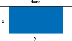
We will first picture the situation and identify the unknowns. Let \( x \) represent the width and \( y \) the length of the dog run, in metres \( (x \gt 0,\ y \gt 0) \).
We know that the area must be \( 35\text{ m}^2\) and \( A = \text{length } \times \text{ width} \).
Therefore, \( xy = 35 \) or \( y = \dfrac{35}{x} \).
The amount of fencing, \( F \), is given by \( F = 2x + y \).
To express \( F \) as function of the width, \( x \), we substitute \( y = \dfrac{35}{x} \) to obtain the rational function
\[ F(x) = 2x + \dfrac{35}{x} \]
Therefore, the function to model the amount of fencing required, \( F \), in terms of the width of the dog run, \( x \), is given by
\[ F(x) = 2x + \dfrac{35}{x},\ x \gt 0\]
This equation can then be written in a simplified form by finding a common denominator and adding the terms:
\[F(x) = \dfrac{2x^2 + 35}{x},\ x \gt 0 \]
- Sketch the graph of this function.
Solution
- Vertical asymptote
To graph the function \( F(x) = \dfrac{2x^2 + 35}{x} \), we will begin by identifying the asymptotes. Since \( x \gt 0 \), we must determine if \( x = 0 \) is a vertical asymptote or a point of discontinuity.
\( F(0) = \dfrac{35}{0} \) is an undefined value. Therefore, the function has a vertical asymptote of \( x = 0 \).
We can also check the behaviour of the function to the right of \(0\) by determining the value of the function at, say, \(x = 0.01\), a point close to \(0\) but slightly greater than \(0\). The result is a large positive value: using the test value \( x = 0.01 \), we see \( F(0.01) = 3500.02 \). So,
\[ \lim_{x \rightarrow 0^+}\dfrac{2x^2 + 35}{x} = + \infty \]
- End behaviour asymptote
The degree of the numerator is one greater than the degree of the denominator; therefore, the function has an oblique asymptote, not a horizontal asymptote.
The original form of the equation, \( F(x) = 2x + \dfrac{35}{x} \), allows us to identify the equation of the oblique asymptote.
As \( x \rightarrow +\infty \), \( \dfrac{35}{x} \rightarrow 0 \), so \( y \rightarrow 2x \). Therefore, \( y = 2x \) is the oblique (or slant) asymptote.
Since \( F(x) = 2x + \dfrac{35}{x} \) and \( \dfrac{35}{x} \) is always positive for \( x \gt 0 \), then \( F(x) \gt 2x \) on the domain of this function, so the curve approaches the oblique asymptote from above.
- Table of values
We now determine some points to complete the sketch of the graph \( F(x) = \dfrac{2x^2 + 35}{x} \).
| \(x\) |
\(F(x)\) |
| \(1\) |
\(37\) |
| \(2\) |
\(21.5\) |
| \(3\) |
\(17.6\) |
| \(4\) |
\(16.75\) |
| \(5\) |
\(17\) |
| \(6\) |
\(17.83\) |
If we consider what we know so far, the curve of this function lies between the \(y\)-axis and the oblique asymptote. A minimum point must occur somewhere along the curve. We will identify several points to help determine an approximate turning point and complete a sketch of the graph.
- Estimate, to \(1\) decimal place of accuracy, the width of the dog run that will minimize the amount of fencing required.
Solution
To estimate the dimensions of the dog run that will require the least amount of fencing, we will consider the table.
| \(x\) |
\(F(x)\) |
| \(3\) |
\(17.6\) |
| \(4\) |
\(16.75\) |
| \(5\) |
\(17\) |
It appears that a minimum value appears somewhere between \(x=3\) and \(x=5\), as the minimum value of \(f(x)\) in the table occurs at \(x=4\).
The minimum amount of fencing may be \( 16.75\text{ m}\) when the width is \(4\text{ m}\).
However, to ensure this claim (within an accuracy of \(1\) decimal place), values on each side of \(4\) (to one decimal place) must be greater than the value \(16.75\).
| \(x\) |
\(F(x)\) |
| \(3\) |
\(17.6\) |
| \(3.9\) |
\(16.774359\) |
| \(4\) |
\(16.75\) |
| \(4.1\) |
\(16.736585\) |
| \(4.2\) |
\(16.733333\) |
| \(4.3\) |
\(16.739535\) |
| \(5\) |
\(17\) |
The amount of fencing required when the width is \(3.9\) is slightly more than \(16.75\). However, when the width is \(4.1\text{ m}\), the amount is slightly less. We must continue by checking \(f(x)\) when the width is \(4.2\). The amount of fencing decreases again. When the width is \(4.3\), we see an increase in the amount of fencing required.
Thus, to one decimal place accuracy, a dog run with a width of \( 4.2\text{ m}\) will require the least amount of fencing.
The amount of fencing required in total is approximately \( 16.7\text{ m}\).
In Summary
You may wish to take a moment to review the key ideas covered in this module and summarised here.
Consider a rational function \( y = \dfrac{g(x)}{h(x)},\ h(x) \neq 0 \) and the degree of \(h(x) \geq 1\).
- If the degree of \( g(x) \) is less than the degree of \( h(x) \), then \( y = 0 \) is the horizontal asymptote of the function.
- If the degree of \( g(x) \) equals the degree of \( h(x) \), then \( y = \dfrac{a}{b} \) is the horizontal asymptote of the function, where \( a \) and \( b \) are the coefficients of the highest degree term in the numerator and denominator, respectively.
- If the degree of \( g(x) \) is greater than the degree of \( h(x) \), there is no horizontal asymptote.
If the degree of \( g(x) \) is exactly one greater than the degree of \( h(x) \), then the function has an oblique asymptote.
Use long division to express the equation of the function in the form \( y = ax + b + \dfrac{r(x)}{h(x)} \), where \( ax + b,\ a \neq 0 \), is the quotient and \( r(x) \) is the remainder.
The oblique (or slant) asymptote is given by \( y = ax + b \).
- A rational function may intersect its horizontal or oblique (or slant) asymptote but will never cross its vertical asymptotes.
- Since the value of a limit provides information near, but not at, a specific value of \( x \), limits are often used when analyzing a function near its asymptotes.
In the next two modules concerned with graphing rational functions, we will employ limit notation and our understanding of asymptotes as we analyse and graph a variety of rational functions.