Logarithmic Functions Alternative Format
Lesson Part 1
Introduction
Logarithms were first introduced by John Napier in the \(17^{\textrm{th}}\) century for the purpose of simplifying calculations.
This was accomplished with the development of logarithmic tables and, soon after, with logarithmic scales on a slide rule.
With the introduction of the scientific calculator in the mid-1970s, this application of logarithms for computations became somewhat obsolete; however, logarithms are still used today in many areas such as
- scientific formulas and scales (the pH scale in chemistry and the Richter scale for measuring and comparing the intensity of earthquakes),
- astronomy (order of magnitude calculations comparing relative size of massive bodies),
- modelling and solving problems involving exponential growth and decay, and
- many areas of calculus.
We will begin our study of logarithms by introducing and exploring the logarithmic function.
The logarithmic function is simply the inverse of the exponential function.
Consider the exponential function,
\[y = c^x, c \gt 0, c \neq 1\]
To obtain the inverse of this function, we interchange the \(x\) and \(y\)-coordinates.
\[x = c^y\]
The next step is usually to solve for \(y\) to express the function in a standard form. This will require the use of logarithms. A logarithm will reverse or undo the operation of exponentiation. We will discuss this in more detail later in this module.
\[y = log_c(x), c \gt 0, c \neq 1\]
Since \(c \gt 0\), \(c \neq 1\) for the exponential function, the same condition applies to \(c\) for this logarithmic form of the equation.
If \(f(x) = c^x,~ c \gt 0,~ c \neq 1\),
then \(f^{-1}(x) = \log_{c}(x), ~c \gt 0, ~c \neq 1 \).
What Is a Logarithm?
Before we study the graph of a logarithmic function, we must first understand what a logarithm is. The logarithmic equation \(y = \log_{c}(x)\) is just the exponential equation in a different form.
That is,
\[y = \log_{c}(x) \quad \Leftrightarrow \quad x = c^y~\text{where}~c > 0, ~c \neq 1\]
Equivalent Forms
Using these equivalent forms, we can then convert the following exponential statements,
\[ \begin{align*} 125 = 5^3 \quad &\Leftrightarrow \quad \log_{5}(125) = 3 \\ \frac{1}{36} = 6^{-2} \quad &\Leftrightarrow \quad \log_{6}\left(\frac{1}{36}\right) = -2 \end{align*} \]
We can also start with the logarithmic form and convert to exponential form.
\[ \log_{4}(32) = \frac{5}{2} \quad \Leftrightarrow \quad 32 = 4^{\frac{5}{2}} \]
In general, let's consider
\[\log_{\textcolor{BrickRed}{c}}{(\textcolor{NavyBlue}{m})} = \textcolor{Mulberry}{n}\]
The base of the logarithm is \(\textcolor{BrickRed}{c}\).
The value of the logarithm, \(\textcolor{Mulberry}{n}\), is the exponent to which the base, \(\textcolor{BrickRed}{c}\), must be raised to yield the value of \(\textcolor{NavyBlue}{m}\).
Thus, \(\textcolor{NavyBlue}{m} = \textcolor{BrickRed}{c}^{\textcolor{Mulberry}{n}}\), so \(\textcolor{NavyBlue}{m}\) is the value of the power. \(\textcolor{NavyBlue}{m}\) is also referred to as the argument of the logarithm.
Lesson Part 2
Examples
Think of a logarithm as an exponent. Let's apply this knowledge to evaluate some logarithms.
Example 1
Evaluate \( \log_{3}(81) \).
Solution
Here \(3\) is the base, and \(81\) is the value of the power, or the argument, and we must determine the exponent.
We ask: “\(3\) raised to what exponent will produce \(81\)?”
\[ \begin{align*} 3^{?} &= 81 \\ 3^4 &= 81 \end{align*} \]
Thus, \(\log_{3}(81) = 4 \).
Example 2
Evaluate \(\log_{25}(5) \).
Solution
Here we ask: “\( 25\) raised to what exponent will produce \(5\)?”
\[ \begin{align*} 25^{?} &=5 \\ \sqrt{25} &= 5 \\ 25^{\frac{1}{2}} &= 5 \end{align*} \]
Thus, \( \log_{25}(5) = \dfrac{1}{2}\).
Check Your Understanding A and B
These questions are not included in the Alternative Format, but can be accessed in the Review section of the side navigation.
Example 3
Evaluate \(\log_{4}(8\sqrt{2}) \).
Solution
For more complicated logarithmic expressions, we may wish to set the logarithm equal to a variable, say \( n \), express the statement in exponential form, and solve the equivalent exponential equation.
Let \(\log_{4}(8\sqrt{2}) = n \).
Then,
\[ 4^n = 8 \sqrt{2} \]
Here the base numbers, \(4\), \(8\), and \(\sqrt2\), can be expressed as powers of \(2\).
\[ (2^2)^n = 2^3\left(2^{\frac{1}{2}}\right) \]
Using exponent laws, we can simplify to a single power of \(2\) on each side of the equation.
\[ \begin{align*} 2^{2n} &= 2^{3 + \frac{1}{2}} \\ 2^{2n} &= 2^{\frac{7}{2}} \end{align*} \]
Two powers of \(2\) are equal when their exponents are equal. Thus,
\[ \begin{align*} 2n &= \dfrac{7}{2} \\ n &= \dfrac{7}{4} \end{align*} \]
Therefore,
\[\log_{4}\left(8\sqrt{2}\right) = \dfrac{7}{4} \]
Check Your Understanding C
This question is not included in the Alternative Format, but can be accessed in the Review section of the side navigation.
Lesson Part 3
Exponential and Logarithmic Functions
Let's now examine the behaviour of the graphs of logarithmic functions.
Consider the graph of \(y = \log_{2}(x)\).
We will use the fact that this logarithmic function is the inverse of the exponential function \( y = 2^x \).
Exponential Function
We begin with the function \(f(x) = 2^{x}\).
\(y= 2^x\) has domain \( \{x \mid x \in \mathbb{R} \} \).
From a table of values, we can produce the graph of the function, one that we are already familiar with.
| \(x\) |
\(y = 2^x\) |
\((x, y)\) |
| \(-3\) |
\(\frac{1}{8}\) |
\( \left(-3, \frac{1}{8}\right)\) |
| \(-2\) |
\(\frac{1}{4}\) |
\(\left(-2, \frac{1}{4}\right)\) |
| \(-1\) |
\(\frac{1}{2}\) |
\( \left(-1, \frac{1}{2}\right)\) |
| \(0\) |
\(1\) |
\((0, 1)\) |
| \(1\) |
\(2\) |
\((1, 2)\) |
| \(2\) |
\(4\) |
\((2, 4)\) |
| \(3\) |
\(8\) |
\((3, 8)\) |
| \(4\) |
\(16\) |
\((4, 16)\) |
The inverse of \(y=2^x\) is given by \(x=2^y\), obtained by interchanging the variables, \(x\) and \(y\).
Expressing \(x=2^y\) in logarithmic form, we have \(y=\log_{2} (x)\).
One way to graph \(y = \log_{2}(x) \) is to interchange the \( x \) and \(y\) coordinates of each point on \( y = 2^x \) to obtain a corresponding point on its inverse.
| \[ \begin{gather*} y = 2^x \\ (x, y) \end{gather*} \] |
\[ \begin{gather*} y = \log_{2}(x) \\ (x, y) \end{gather*} \] |
| \( \left(-3, \frac{1}{8}\right)\) |
\(\left(\frac{1}{8}, -3\right)\) |
| \( \left(-2, \frac{1}{4}\right)\) |
\(\left(\frac{1}{4}, -2\right)\) |
| \(\left(-1, \frac{1}{2}\right)\) |
\(\left(\frac{1}{2}, -1\right)\) |
| \((0, 1)\) |
\((1, 0)\) |
| \((1, 2)\) |
\((2, 1)\) |
| \((2, 4)\) |
\((4, 2)\) |
| \( (3, 8)\) |
\((8, 3)\) |
| \((4, 16)\) |
\((16, 4)\) |
We now plot these points to obtain the graph of \(y=\log_{2} x\).
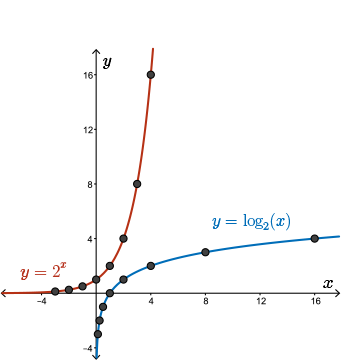
The coordinates of these points support our understanding of logarithms.
Using the point \(\left (\frac{1}{8},-3 \right )\), we have \(\log_{2} \left (\frac{1}{8}\right ) = -3\), which follows from \(2^{-3}=\frac{1}{8}\).
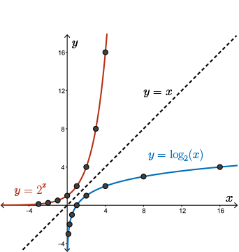
The graph of the inverse of a function is the reflection of the original function in the line \( y = x \).
Note that not all functions have an inverse function.
In this case, however, \( y = \log_{2}(x) \) is a function since each value of \( x \) in its domain produces exactly one value for \( y\) (that is, its graph passes the vertical line test).
Thus, using function notation,
\[f^{-1} (x)=\log_{2} (x)\]
The graph of \(y=2^x\) has a horizontal asymptote of \(y=0\), the \(x\)-axis.
The graph of \( y = \log_{2}(x) \) has a vertical asymptote of \(x = 0\), the \(y\)-axis.
The domain of the exponential function is the range of the logarithmic function, the set of all real numbers. The range of the exponential function is the domain of the logarithmic function, the set of all real values greater than \(0\).
| |
Domain |
Range |
| \(y = 2^x\) |
\(\{x \mid x \in \mathbb{R} \}\) |
\(\{ y \mid y \gt 0, ~y \in \mathbb{R} \}\) |
| \(y = \log_{2}(x)\) |
\(\{ x \mid x \gt 0,~ x \in \mathbb{R} \}\) |
\(\{ y \mid y \in \mathbb{R} \}\) |
The graphs of both functions, \( y = 2^x\) and \(y = \log_{2}(x)\), are increasing.
Create the graph of \(y = \log_{\frac{1}{2}}(x) \) using the graph of \( y = \left(\frac{1}{2}\right)^x \). Compare the features of the two graphs.
Determine points on \( y = \left(\frac{1}{2} \right)^x \) and then plot them on the graph.
| \begin{gather*}y = \left(\tfrac{1}{2} \right)^x \\ (x, y) \end{gather*} |
\begin{gather*}y = \log_{\frac{1}{2}}(x) \\ (x, y) \end{gather*} |
| \( (-3, 8)\) |
|
| \( (-2, 4)\) |
|
| \((-1, 2)\) |
|
| \((0, 1)\) |
|
| \(\left(1, \frac{1}{2}\right)\) |
|
| \(\left(2, \frac{1}{4}\right)\) |
|
| \( \left(3, \frac{1}{8}\right)\) |
|
| \(\left(4, \frac{1}{16}\right)\) |
|
Interchange the coordinates of the points on \( y = \left(\frac{1}{2} \right)^x \) to obtain the corresponding points on \( y = \log_{\frac{1}{2}}(x) \).
Plot the corresponding points to obtain the graph of \( y = \log_{\frac{1}{2}}(x)\).
| \(\begin{gather*}y = \left(\tfrac{1}{2} \right)^x \\ (x, y) \end{gather*}\) |
\(\begin{gather*}y = \log_{\frac{1}{2}}(x) \\ (x, y) \end{gather*}\) |
| \( (-3, 8)\) |
\((8, -3)\) |
| \( (-2, 4)\) |
\((4, -2)\) |
| \((-1, 2)\) |
\((2, -1)\) |
| \((0, 1)\) |
\((1, 0)\) |
| \(\left(1, \frac{1}{2}\right)\) |
\(\left(\frac{1}{2}, 1\right)\) |
| \(\left(2, \frac{1}{4}\right)\) |
\(\left(\frac{1}{4}, 2\right)\) |
| \( \left(3, \frac{1}{8}\right)\) |
\(\left(\frac{1}{8}, 3\right)\) |
| \(\left(4, \frac{1}{16}\right)\) |
\(\left(\frac{1}{16}, 4\right)\) |
The graph of \( y = \log_{\frac{1}{2}}(x) \) is the reflection of the graph of \(y = \left(\frac{1}{2}\right)^x \) in the line \( y = x \).
\( y = \log_{\frac{1}{2}}(x) \) has a vertical asymptote of \( x = 0 \).
\(y = \left(\frac{1}{2}\right)^x \) has a horizontal asymptote of \(y = 0 \).
In this case, both \( y = \left( \frac{1}{2} \right)^x \) and \(y = \log_{\frac{1}{2}}(x) \) are decreasing functions.
The domain and range of the logarithmic function, base \(\frac{1}{2}\), is the same as the domain and range of the logarithmic function, base \(2\), the domain being the set of all real values greater than \(0\) and the range the set of all real values.
| Function |
Domain |
Range |
| \(y = \left(\frac{1}{2} \right)^x\) |
\(\{x \mid x \in \mathbb{R} \}\) |
\(\{ y \mid y \gt 0, \ y \in \mathbb{R} \}\) |
| \(y = \log_{\frac{1}{2}}(x)\) |
\(\{ x \mid x \gt 0, \ x \in \mathbb{R} \}\) |
\(\{ y \mid y \in \mathbb{R} \}\) |
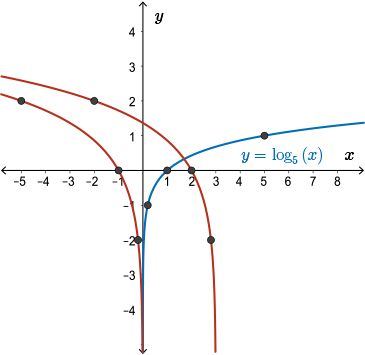
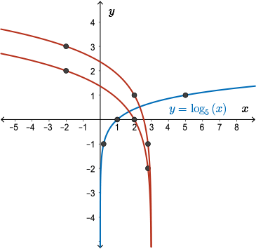
How does the graph of \( y = \log_{\frac{1}{2}}(x) \) compare to the graph of \(y = \log_{2}(x)\)?
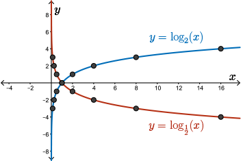
Placing the graph of each function on the same set of axes, we see \( y = \log_{\frac{1}{2}}(x) \) is a reflection of \(y = \log_{2}(x) \) in the \(x\)-axis.
Using our understanding of transformations, we can say
\[\log_{\frac{1}{2}}(x) = -\log_{2}(x)\]
We will prove this algebraically, in the next module, after studying the laws of logarithms.
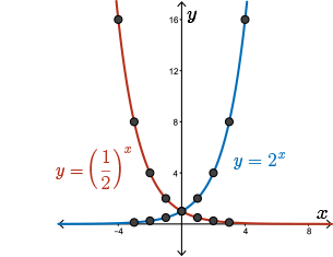
Recall that the graphs of corresponding exponential function, \(y = 2^x\) and \(y = \left(\frac{1}{2}\right)^x\), studied earlier in this unit, are reflections of each other in the \( y \)-axis.
That is,
\[2^x = \left(\frac{1}{2}\right)^{-x}\]
This is easily proven using the exponent laws:
\[\left(\frac{1}{2}\right)^{-x} = \left[ \left(\frac{1}{2} \right)^{-1} \right]^x = 2^x\]
We have explored the behaviour of a logarithmic function base \(2\) and base \(\frac{1}{2}\). Use the first investigation provided in this module to investigate the behaviour of the logarithmic function as the value of the base changes.
Investigation 1
See Investigation 1 in the side navigation.
Lesson Part 4
Let's summarize our observations.
General Observations
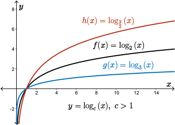
The graphs of logarithmic functions of the form \( y = \log_{c}(x), ~c \gt 0, ~c \neq 1 \), have
- domain \( \{x \mid x \gt 0,~x \in \mathbb{R} \} \) and range \(\{y \mid y \in \mathbb{R} \} \),
- an \(x \)-intercept at \((1, 0) \) and no \( y \)-intercept, and
- a vertical asymptote of \(x = 0 \) (the \(y\)-axis).
The graph of a logarithmic function where \(c \gt 1 \) is always increasing. The greater the value of the base, \( c \), the slower the curve increases as \(x\) increases.
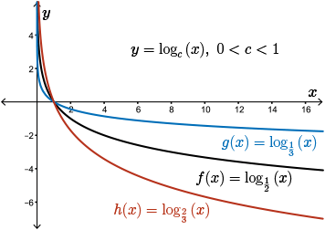
The graph of a logarithmic function where \( 0 \lt c \lt1 \) is always decreasing. The smaller the value of the base, \(c, \) the slower the curve decreases as \(x\) increases.
Check Your Understanding D
This question is not included in the Alternative Format, but can be accessed in the Review section of the side navigation.
Transformations of Logarithmic Functions
Now that we are familiar with the behaviour and shape of basic logarithmic functions, let's take a look at transformations of these functions.
The effect of each parameter \( \textcolor{BrickRed}{a}\), \(\textcolor{NavyBlue}{b}\), \(\textcolor{Mulberry}{h}\), and \( \textcolor{Violet}{k} \) in the equation \( y = \textcolor{BrickRed}{a}\log_{c}(\textcolor{NavyBlue}{b}(x - \textcolor{Mulberry}{h})) + \textcolor{Violet}{k}\) in transforming \(y = \log_c(x)\) is the same as the effect each has on other functions studied previously.
A summary of the effects is outlined here for your review.
The parameters \( \textcolor{BrickRed}{a}\), \(\textcolor{NavyBlue}{b}\), \(\textcolor{Mulberry}{h}\), and \( \textcolor{Violet}{k} \) in the equation \( y = \textcolor{BrickRed}{a}\log_{c}(\textcolor{NavyBlue}{b}(x - \textcolor{Mulberry}{h})) + \textcolor{Violet}{k}\) correspond to the following transformations:
- If \( \textcolor{BrickRed}{a} \lt 0, ~y = \log_{c}(x)\) is reflected in the \( x \)-axis.
- \( y = \log_{c}(x) \) is stretched vertically about the \( x \)-axis by a factor of \(\lvert \textcolor{BrickRed}{a} \rvert\).
- If \(\textcolor{NavyBlue}{b} \lt 0, ~y = \log_{c}(x) \) is reflected in the \( y\)-axis.
- \(y = \log_{c}(x) \) is stretched horizontally about the \( y \)-axis by a factor of \( \dfrac{1}{\lvert \textcolor{NavyBlue}{b} \rvert} \).
- \(y = \log_{c}(x) \) is translated horizontally \( \textcolor{Mulberry}{h} \) units.
If \(\textcolor{Mulberry}{h} \gt 0\), then \(y=\log_{c}(x)\) is translated right.
If \(\textcolor{Mulberry}{h} \lt 0\), then \(y=\log_{c}(x)\) is translated left.
- \(y = \log_{c}(x) \) is translated vertically \( \textcolor{Violet}{k} \) units.
If \(\textcolor{Violet}{k} \gt 0\), then \(y=\log_{c}(x)\) is translated up.
If \(\textcolor{Violet}{k} \lt 0\), then \(y=\log_{c}(x)\) is translated down.
The transformation of each point is defined by the mapping \((x,y) \rightarrow \left(\dfrac{1}{\textcolor{NavyBlue}{b}}x + \textcolor{Mulberry}{h}, ~\textcolor{BrickRed}{a}y + \textcolor{Violet}{k} \right) \).
A well, an investigation has been included in this module for you to investigate and verify the effects of these parameters on transforming logarithmic functions.
Check Your Understanding E
This question is not included in the Alternative Format, but can be accessed in the Review section of the side navigation.
Investigation 2
See Investigation 2 in the side navigation.
Lesson Part 5
Examples
Example 4
Let's now consider a transform of a logarithmic function.
a. Graph the function \( f(x) = 2\log_{5}(3 - x) + 1 \). Identify the domain, range, and any asymptote of the function. Is the function increasing or decreasing?
b. Determine the equation \( y = f^{-1}(x) \) and sketch its graph.
Solution Part a
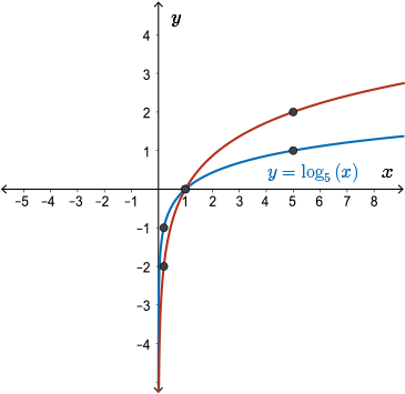
Starting with the graph of \( y = \log_{5}(x) \), we will use our knowledge of transformations to obtain the graph of \(f(x)\).
We are familiar with the basic shape of the graph of this function, but we will use a quick table of values to find the exact location of the curve.
First note that the domain of the function is \(\{x \mid x \gt 0, \ x \in \mathbb{R} \} \).
By selecting powers of \(5\) for \(x\), we can quickly identify the corresponding \(y\) value.
| \(x\) |
\(y = \log_{5}(x)\) |
| \(\frac{1}{5}\) |
\(\log_{5}\left(\frac{1}{5}\right)=-1\) |
| \(1\) |
\(\log_{5}(1)=0\) |
| \(5\) |
\(\log_{5}(5)=1\) |
| \(25\) |
\(\log_{5}(25)=2\) |
Using the first three points, we can graph the function.
To correctly identify the transformations that must be applied to \(y = \log_{5}(x)\) to achieve \(f(x) = 2\log_{5}(3 - x) + 1\), we will first factor the coefficient of \(x\), in this case, the \(-1\), from the argument \((3 - x)\). Therefore,
\[f(x) = 2\log_{5}[-(x - 3)] + 1\]
We may obtain the graph of \( f(x) \) from the graph of \(y = \log_{5}(x) \) by applying the following transformations, in order:
First, apply a vertical stretch about the \( x \)-axis by a factor of \(2\).
Next, apply a reflection in the \( y \)-axis.
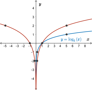
Then, apply a horizontal translation right \(3\) units.
Finally, apply a vertical translation up \(1\) unit.
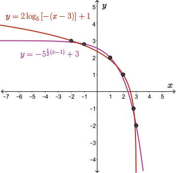
\(f(x) = 2\log_{5}[-(x - 3)] + 1\)
The domain is \( \{x \mid x \lt 3, \ x \in \mathbb{R} \} \).
This is seen graphically but can be obtained algebraically since
\[ \begin{align*} -(x - 3) &\gt 0 \\ x - 3 &\lt 0 \\ x &\lt 3 \end{align*} \]
The range is \( \{ y \mid y \in \mathbb{R} \} \).
The function is decreasing and has a vertical asymptote of \( x = 3 \).
Solution Part b
To determine the equation of the inverse of \( f(x) = 2\log_{5}[-(x - 3)] + 1 \), we must interchange the \( x \) and \( y \) variables in the equation of \( f(x) \) and solve for \(y\).
Inverse:
\[ \begin{align*} x &= 2\log_{5}[-(y - 3)] + 1 \\ x - 1 &= 2\log_{5}[-(y - 3)] \\ \dfrac{x - 1}{2} &= \log_{5}[-(y - 3)] \\ \textcolor{Mulberry}{\dfrac{x - 1}{2}} &= \log_{\textcolor{BrickRed}{5}}[\textcolor{NavyBlue}{-(y - 3)}] \\ \textcolor{BrickRed}{5}^{\textcolor{Mulberry}{\frac{x - 1}{2}}} &= \textcolor{NavyBlue}{-(y - 3)} \\ y &= -5^{\frac{x - 1}{2}} + 3 \\ \therefore f^{-1}(x) &= -5^{\frac{x - 1}{2}} + 3 \end{align*} \]
The graph of \( f^{-1}(x) = -5^{\frac{x - 1}{2}} + 3 \) can be obtained by
- interchanging the \(x\) and \(y\) coordinates of the points on \( f(x) \) to obtain points on \( f^{-1} {(x)}\),
- reflecting the graph of \( f(x) = 2\log_{5}[-(x - 3)] + 1 \) in the line \( y = x \), or
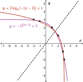
- applying the appropriate transformations to the graph of \( y = 5^x \)
- a reflection in the \(x\)-axis
- a horizontal stretch about the \(y\)-axis by a factor of \(2\)
- a horizontal translation right \(1\) unit
- a vertical translation up \(3\) units
Check Your Understanding F and G
These questions are not included in the Alternative Format, but can be accessed in the Review section of the side navigation.
Summary
- The value of a logarithm is an exponent. The statement \( \log_{c}(m) = n \) is equivalent to \( c^n = m \).
- The inverse of \( y = c^x, ~c \gt 0,~ c \neq 1 \) is \( y = \log_{c}(x), ~c \gt 0, ~c \neq 1 \). Their graphs are reflections of each other in the line \( y = x \).
- The function \( y = \log_{c}(x),~ c \gt 0, ~c \neq 1 \)
- has a domain of \( \{x\mid x \gt 0,\ x \in \mathbb{R} \} \) and a range of \(\{y \mid y \in \mathbb{R} \} \),
- has an \( x \)-intercept at \( (1, 0) \) and a vertical asymptote of \( x = 0 \), the \(y\)-axis, and
- is increasing when \( c \gt 1 \) and decreasing when \(0 \lt c \lt 1 \).
- The parameters \( \textcolor{BrickRed}{a}, \textcolor{NavyBlue}{b}, \textcolor{Mulberry}{h} \), and \( \textcolor{Violet}{k} \) of \(y = \textcolor{BrickRed}{a}\log_{c}{[\textcolor{NavyBlue}{b}(x - \textcolor{Mulberry}{h})]} + \textcolor{Violet}{k} \) correspond to transformations that map points, \((x,y)\), on \(y=c^x\) to \( \left(\frac{1}{\textcolor{NavyBlue}{b}}x + \textcolor{Mulberry}{h}, \ \textcolor{BrickRed}{a}y + \textcolor{Violet}{k} \right) \); exactly as they did for functions of the form \(y = \textcolor{BrickRed}{a}f[\textcolor{NavyBlue}{b}(x - \textcolor{Mulberry}{h})] + \textcolor{Violet}{k} \).